
import os
import numpy as np
import pandas as pd
import plotnine as p9
from Bio import Entrez
import geopandas as gpd
from collections import defaultdict
from itables import init_notebook_mode, show
from mizani.formatters import percent_formatJapan Aerobiome Sampling 2014-2018
Analysis of HVS metagenomic data from Noto, Toyama and Kumamoto
Preamble
Show code imports and presets
In this section we load the necessary libraries and set the global parameters for the notebook. It’s irrelevant for the narrative of the analysis but essential for the reproducibility of the results.
Code imports
Presets
# Matplotlib settings
import matplotlib.pyplot as plt
from matplotlib_inline.backend_inline import set_matplotlib_formats
plt.rcParams['font.family'] = 'Georgia'
plt.rcParams['svg.fonttype'] = 'none'
set_matplotlib_formats('retina')
plt.rcParams['figure.dpi'] = 300

# Plotnine settings (for figures)

p9.options.set_option('base_family', 'Georgia')

p9.theme_set(
    p9.theme_bw()
    + p9.theme(panel_grid=p9.element_blank(),
               legend_background=p9.element_blank(),
               panel_grid_major=p9.element_line(size=.5, linetype='dashed',
                                                alpha=.15, color='black'),
               plot_title=p9.element_text(ha='center'),
               dpi=300
    )
)

# This is needed to display the interactive tables
init_notebook_mode(all_interactive=True)Entrez.email = "alejandro.fontal@isglobal.org"Introduction
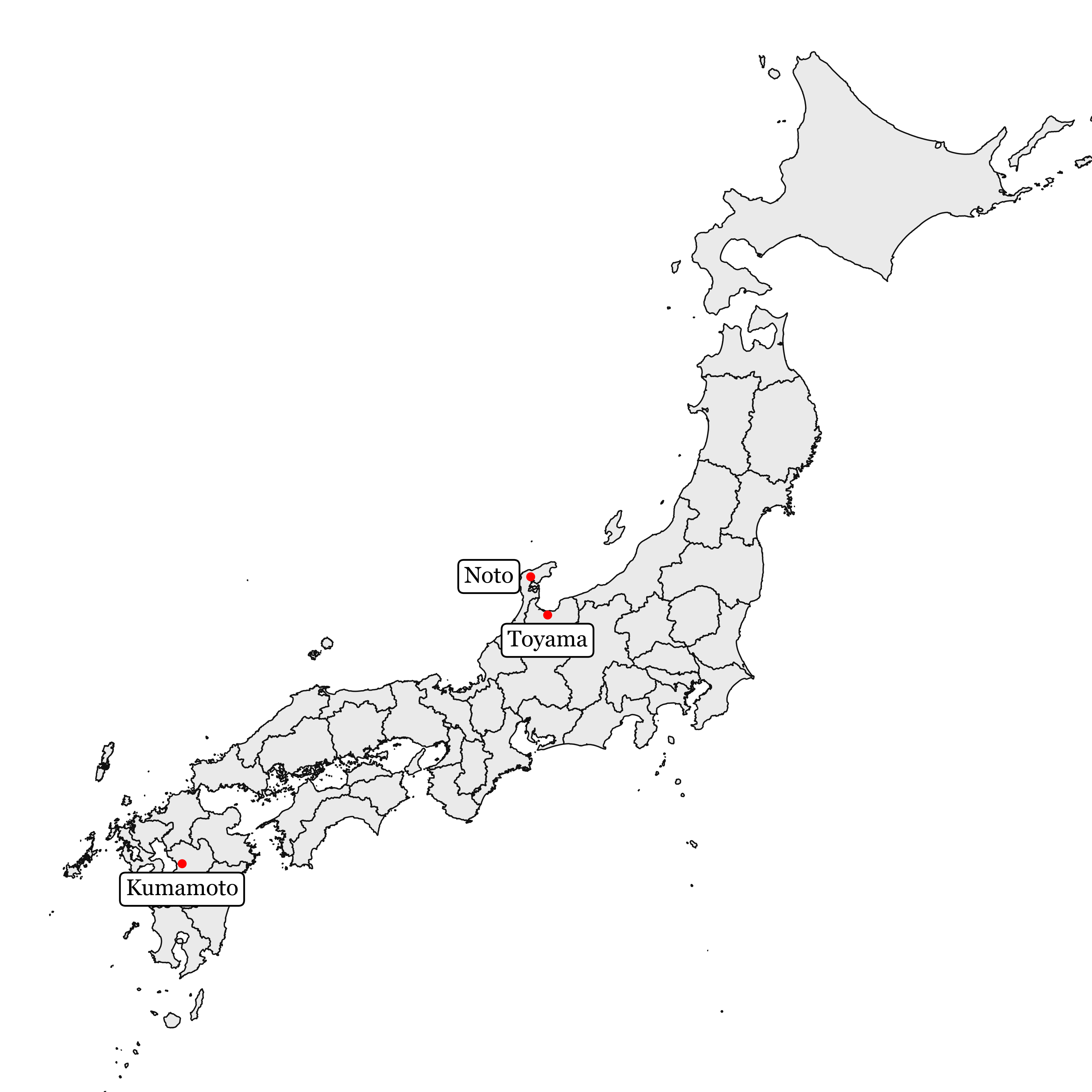
In this notebook we will analyze the metagenomic data from 3 different sampling campaigns made in Japan. The data was collected in the cities of Noto, Toyama and Kumamoto between 2014 and 2018.
The DNA used as source for the metagenomic analysis was extracted from quartz filters which were used to capture the particles in the air for different periods of time with a high volume sampler (HVS) with either a 2.5 or 10 µm cutoff.
The locations in the map of Japan are the following:
Show Code
print(' ')
japan_shape = gpd.read_file('../../kd-spatial-ts/data/shapefiles/jpn_admbnda_adm1_2019.zip')
toyama_coords = (36.7, 137.2)
kumamoto_coords = (32.8, 130.7)
noto_coords = (37.3, 136.9)

(japan_shape
 .query('ADM1_PCODE != "JP47"')
 .pipe(lambda dd: p9.ggplot(dd)
       + p9.geom_map(alpha=.1, size=.3)
       + p9.xlim(None, 146)
       + p9.ylim(30, None)
       + p9.theme_void()
       + p9.annotate('point', x=toyama_coords[1], y=toyama_coords[0], color='red', size=1)
       + p9.annotate('point', x=kumamoto_coords[1], y=kumamoto_coords[0], color='red', size=1)
       + p9.annotate('point', x=noto_coords[1], y=noto_coords[0], color='red', size=1)
       + p9.annotate('label', x=toyama_coords[1], y=toyama_coords[0], label='Toyama', size=9,
                      color='black', ha='center', nudge_y=-.4, alpha=1)
            + p9.annotate('label', x=kumamoto_coords[1], y=kumamoto_coords[0], label='Kumamoto', size=9,
                              color='black', ha='center', nudge_y=-.4, alpha=1)
            + p9.annotate('label', x=noto_coords[1], y=noto_coords[0], label='Noto', size=9,
                              color='black', ha='right', nudge_x=-.3, alpha=1)
       + p9.theme(figure_size=(6, 6), dpi=300)
 )
) 
The data for Noto was taken from 2014 to 2016 and was analyzed via 16S and ITS amplicon sequencing.
The data for Kumamoto and Toyama was taken from 2017 to 2018 and was analyzed with PacBio long reads.
The two methods are different and the data is not directly comparable, but we can still analyze the data to find interesting patterns.
The main aim here is to (1) explore the diversity and validity of the diversity of the samples, and (2) explore a potential association between the samples and the incidence of Kawasaki Disease in the regions.
Data Loading and Wrangling
Load data files into dataframes
kumamoto_all = pd.read_csv('../data/clean_results_tables/kumamoto_all_2024db.tsv', sep='\t', skiprows=136)
toyama_all = pd.read_csv('../data/clean_results_tables/toyama_all_2024db.tsv', sep='\t', skiprows=148)
noto_all = pd.concat([pd.read_csv('../data/clean_results_tables/noto_all_16S.csv'),
                      pd.read_csv('../data/clean_results_tables/noto_all_ITS.csv')])
The data for Noto already provides the full taxonomy of each ASV, together with the total number of reads for each of the samples, which are already labeled.
The data for Toyama and Kumamoto is in the form of the output of Kraken, which provides the taxonomic ID of each read and the number of reads for each of the samples but in an encoded way. The depth of taxonomy is also provided, so we can choose up to which level we want to analyze the data.
In any case, to get a proper taxonomic value for each read we need to use the Entrez API to retrieve the full taxonomy of each read and append it to the data. We will also have to start by using the annotations in the first lines of the document to match the sample names with the kraken ids.
Defining the kraken to sample id maps
kraken_to_sample_map_toyama = {}
with open('../data/clean_results_tables/toyama_all_2024db.tsv', 'r') as f:
    for line in f.readlines():
        if line.startswith('#S'):
            kraken, sample_id =  line.split('\t')
            kraken_to_sample_map_toyama[kraken[2:]] = sample_id.split('report_')[-1].split('.')[0]

kraken_to_sample_map_kumamoto = {}
with open('../data/clean_results_tables/kumamoto_all_2024db.tsv', 'r') as f:
    for line in f.readlines():
        if line.startswith('#S'):
            kraken, sample_id =  line.split('\t')
            kraken_to_sample_map_kumamoto[kraken[2:]] = sample_id.split('report_')[-1].split('.')[0]
Fetching the taxonomy data from NCBI and wrangling the data tables
def get_taxonomy(tax_id):
    # Fetch the taxonomy data using efetch
    handle = Entrez.efetch(db="taxonomy", id=tax_id, retmode="xml")
    records = Entrez.read(handle)
    relevant_ranks = ['kingdom', 'phylum', 'class', 'order', 'family', 'genus', 'species']
    # Extract taxonomy information
    tax_data = {}
    if records:
        record = records[0]
        # Extract the lineage and scientific name
        tax_data['ScientificName'] = record.get('ScientificName')
        for lineage in record.get('LineageEx', []):
            if lineage['Rank'] in relevant_ranks:
                tax_data[lineage['Rank'].capitalize()] = lineage['ScientificName']
    return tax_data

relevant_toyama = (toyama_all
 .query('taxid.notna()')
 .assign(taxid=lambda dd: dd.taxid.astype(int))
 .query('lvl_type.isin(["D", "K", "P", "C", "O", "F", "G", "S"])')
)

relevant_kumamoto = (kumamoto_all
    .query('taxid.notna()')
    .assign(taxid=lambda dd: dd.taxid.astype(int))
    .query('lvl_type.isin(["D", "K", "P", "C", "O", "F", "G", "S"])')
    )

toyama_ids = relevant_toyama['taxid'].to_list()
kumamoto_ids = relevant_kumamoto['taxid'].to_list()
all_ids = list(set(toyama_ids + kumamoto_ids))

if not os.path.exists('../checkpoints/parsed_taxonomy.csv'):
    all_records_1 = Entrez.read(Entrez.efetch(db="taxonomy",
                                id=all_ids[:len(all_ids) // 2], retmode="xml"))
    all_records_2 = Entrez.read(Entrez.efetch(db="taxonomy",
                                id=all_ids[len(all_ids) // 2:], retmode="xml"))
    all_records = all_records_1 + all_records_2
    relevant_ranks = ['superkingdom', 'kingdom', 'phylum', 'class',
                      'order', 'family', 'genus', 'species']
    parsed_records = defaultdict(list)
    for record in all_records:
        parsed_records['taxid'].append(record['TaxId'])
        parsed_records['rank'].append(record['Rank'])
        try:
            available_ranks = [lineage['Rank'] for lineage in record['LineageEx']]
        except KeyError:
            available_ranks = []
        for rank in relevant_ranks:
            if rank in available_ranks:
                parsed_records[rank.capitalize()].append(
                    [lineage['ScientificName'] for lineage in record['LineageEx']
                    if lineage['Rank'] == rank][0])
            elif rank == record['Rank']:
                parsed_records[rank.capitalize()].append(record['ScientificName'])
            else:
                parsed_records[rank.capitalize()].append(pd.NA)
    parsed_records = pd.DataFrame(parsed_records).assign(taxid=lambda dd: dd.taxid.astype(int))
    parsed_records.to_csv('../checkpoints/parsed_taxonomy.csv', index=False)
else:
    parsed_records = pd.read_csv('../checkpoints/parsed_taxonomy.csv')


taxa = ['Superkingdom', 'Kingdom', 'Phylum', 'Class', 'Order', 'Family', 'Genus', 'Species']

clean_toyama = (relevant_toyama
 .merge(parsed_records)
 .drop(columns=[col for col in relevant_toyama.columns if '_lvl' in col])
 .assign(rank=lambda dd: dd['rank'].str.capitalize())
 .drop(columns=['tot_all', '#perc', 'lvl_type'])
 .melt(taxa + ['taxid', 'name', 'rank'], var_name='sample_id', value_name='reads')
 .assign(sample_id=lambda dd: dd.sample_id.str.split('_').str[0].map(kraken_to_sample_map_toyama))
 .assign(sample_id=lambda dd: dd.sample_id.str.replace('_', '.').str.replace('.1', ''))
 .assign(reads=lambda dd: dd.reads.astype(int))
)

clean_kumamoto = (relevant_kumamoto
    .merge(parsed_records)
    .drop(columns=[col for col in relevant_kumamoto.columns if '_lvl' in col])
    .assign(rank=lambda dd: dd['rank'].str.capitalize())
    .drop(columns=['tot_all', '#perc', 'lvl_type'])
    .melt(taxa + ['taxid', 'name', 'rank'], var_name='sample_id', value_name='reads')
    .assign(sample_id=lambda dd: dd.sample_id.str.split('_').str[0].map(kraken_to_sample_map_kumamoto))
    .assign(sample_id=lambda dd: dd.sample_id.str.replace('_', '.').str.replace('.1', ''))
    .assign(sample_id=lambda dd: dd.sample_id.str[:2] + dd.sample_id.str[2:].str.zfill(3))
    .assign(reads=lambda dd: dd.reads.astype(int))
)clean_toyama| Superkingdom | Kingdom | Phylum | Class | Order | Family | Genus | Species | taxid | name | rank | sample_id | reads |
|---|---|---|---|---|---|---|---|---|---|---|---|---|
|
Loading ITables v2.1.4 from the init_notebook_mode cell...
(need help?) |
Samples Calendar
To be able to understand the data we need to be aware of the duration of the sampling campaigns, the duration and total volume of air filtered in each of the samples, the type of filter used and the hours of the day in which the samples were taken, since we know that each of these factors can influence the composition of the samples.
If we make a simple calendar showing the dates for which we have samples in each of the sites:
Code to wrangle and clean the calendars
def expand_dates(row):
return pd.DataFrame({
'sample_id': row['sample_id'],
'date': pd.date_range(row['start_date'], row['end_date'])
})
dates_17_18 = (pd.date_range('2017-01-01', '2018-12-31', freq='1D')
.rename('date')
.to_frame()
.reset_index(drop=True)
)
samples_info = (pd.read_csv('../data/clean_results_tables/filters_inventory.csv', skiprows=3)
.query('Location=="Toyama"')
.rename(columns={
'Unnamed: 0': 'sample_id',
'Duration (h)': 'duration',
'Sampled air volume (m3)': 'volume',
'Sampling head': 'header',
})
.assign(sample_id=lambda dd: dd.sample_id.str.replace('.1', ''))
.assign(start_date=lambda dd: pd.to_datetime(dd['Initial date'], dayfirst=True))
.assign(end_date=lambda dd: pd.to_datetime(dd['Final date'], dayfirst=True))
.assign(start_dt=lambda dd: pd.to_datetime(dd.start_date.astype(str) + " " + dd['Start time'], errors='coerce'))
.assign(end_dt = lambda dd: dd.start_dt + pd.to_timedelta(dd.duration, unit='h'))
.drop(columns=['Initial date', 'Final date', 'Sampling', 'Start time',
'End time', 'Filter diameter (mm)', 'Location'])
)
sample_dates = (pd.concat(samples_info
.query('header=="PM10"')
.apply(expand_dates, axis=1).to_list()))
pm10_samples = (pd.concat(samples_info
.query('header=="PM10"')
.apply(expand_dates, axis=1).to_list())
.merge(samples_info)
.merge(dates_17_18, how='right', on='date')
.assign(year=lambda dd: dd.date.dt.year + .5)
)
pm25_samples = (pd.concat(samples_info
.query('header=="PM2.5"')
.apply(expand_dates, axis=1).to_list())
.merge(samples_info)
.merge(dates_17_18, how='right', on='date')
.assign(year=lambda dd: dd.date.dt.year)
)
noto_samples = (pd.read_csv('../data/clean_results_tables/filters_inventory.csv', skiprows=3)
.query('Location=="Noto"')
.rename(columns={
'Unnamed: 0': 'sample_id',
'Duration (h)': 'duration',
'Sampled air volume (m3)': 'volume',
'Sampling head': 'header',
})
.assign(sample_id=lambda dd: dd.sample_id.str.replace('.1', ''))
.assign(start_date=lambda dd: pd.to_datetime(dd['Initial date'], dayfirst=True))
.assign(end_date=lambda dd: pd.to_datetime(dd['Final date'], dayfirst=True))
.assign(start_dt=lambda dd: pd.to_datetime(dd.start_date.astype(str) + " " + dd['Start time'], errors='coerce'))
.assign(end_dt = lambda dd: dd.start_dt + pd.to_timedelta(dd.duration, unit='h'))
.drop(columns=['Initial date', 'Final date', 'Sampling', 'Start time',
'End time', 'Filter diameter (mm)', 'Location'])
)
kumamoto_samples = (pd.read_csv('../data/clean_results_tables/filters_inventory.csv', skiprows=3)
.query('Location=="Kumamoto"')
.rename(columns={
'Unnamed: 0': 'sample_id',
'Duration (h)': 'duration',
'Sampled air volume (m3)': 'volume',
'Sampling head': 'header',
})
.assign(sample_id=lambda dd: 'KS' + dd.sample_id.str.replace('.1', '').str[2:].str.zfill(3))
.assign(start_date=lambda dd: pd.to_datetime(dd['Initial date'], dayfirst=True))
.assign(end_date=lambda dd: pd.to_datetime(dd['Final date'], dayfirst=True))
.assign(start_dt=lambda dd: pd.to_datetime(dd.start_date.astype(str) + " " + dd['Start time'], errors='coerce'))
.assign(end_dt = lambda dd: dd.start_dt + pd.to_timedelta(dd.duration, unit='h'))
.drop(columns=['Initial date', 'Final date', 'Sampling', 'Start time',
'End time', 'Filter diameter (mm)', 'Location'])
)
noto_calendar = (noto_samples
.assign(date=lambda dd: dd.start_date)
.merge(pd.date_range('2014-01-01', '2016-12-31', freq='1D')
.rename('date').to_frame().reset_index(drop=True),
how='right', on='date')
.assign(year=lambda dd: dd.date.dt.year)
.assign(dayofyear=lambda dd: dd.date.dt.dayofyear)
.assign(location='Noto (2014-2016)')
)
toyama_calendar = (pd.concat([pm10_samples, pm25_samples])
.assign(dayofyear=lambda dd: dd.date.dt.dayofyear)
.assign(location='Toyama (2017-2018)')
)
kumamoto_calendar = (pd.concat(kumamoto_samples
.apply(expand_dates, axis=1)
.to_list())
.merge(kumamoto_samples)
.merge(dates_17_18, how='right', on='date')
.assign(year=lambda dd: dd.date.dt.year)
.assign(dayofyear=lambda dd: dd.date.dt.dayofyear)
.assign(location='Kumamoto (2017-2018)')
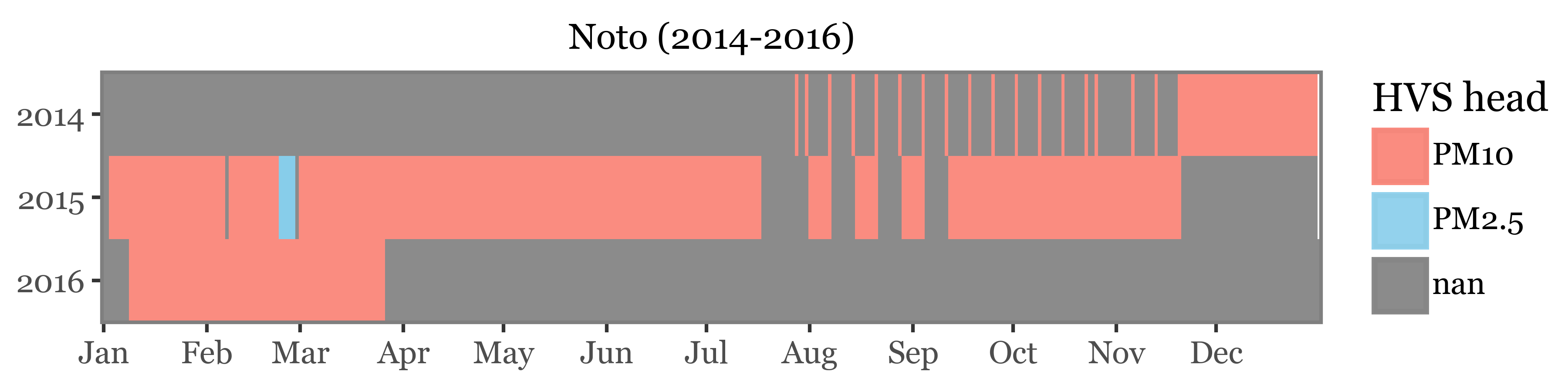
)For noto, we have a mix of daily samples, weekly samples, and subdaily samples taken during an intensive campaign. All samples were taken using a 10 µm header except for the intensive campaign, which used a 2.5 µm header:
Show Code
(noto_calendar
 .pipe(lambda dd: p9.ggplot(dd)
  + p9.aes('dayofyear', 'year')
  + p9.geom_tile(p9.aes(fill='header'), alpha=.9))
  + p9.scale_y_reverse(breaks=[2014, 2015, 2016])
  + p9.scale_fill_manual(['salmon', 'skyblue'])
  + p9.scale_x_continuous(
    breaks=[1, 32, 60, 91, 121, 152, 182, 213, 244, 274, 305, 335],
    labels=['Jan', 'Feb', 'Mar', 'Apr', 'May', 'Jun', 'Jul',
            'Aug', 'Sep', 'Oct', 'Nov', 'Dec'])
  + p9.labs(x='', y='', title='Noto (2014-2016)')
  + p9.coord_fixed(expand=False, ratio=25)
  + p9.guides(fill=p9.guide_legend(title='HVS head'))
  + p9.theme(panel_grid=p9.element_blank(),
             figure_size=(6, 1.5),
             plot_title=p9.element_text(size=10),
)
)
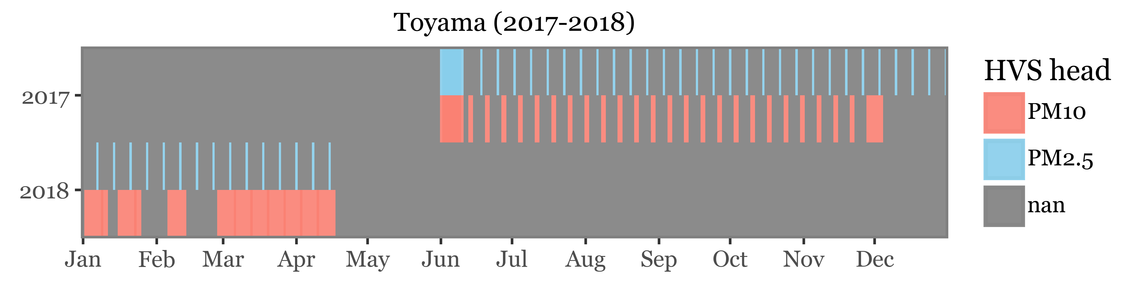
For Toyama, we have a mix of daily and weekly samples taken with a 2.5 and 10 µm header, intercalated:
Show Code
(toyama_calendar
 .pipe(lambda dd: p9.ggplot(dd)
  + p9.aes('dayofyear', 'year')
  + p9.geom_tile(p9.aes(fill='header'), alpha=.9))
  + p9.scale_y_reverse(breaks=[2017.25, 2018.25], labels=['2017', '2018'])
  + p9.scale_fill_manual(['salmon', 'skyblue'])
  + p9.scale_x_continuous(
    breaks=[1, 32, 60, 91, 121, 152, 182, 213, 244, 274, 305, 335],
    labels=['Jan', 'Feb', 'Mar', 'Apr', 'May', 'Jun', 'Jul',
            'Aug', 'Sep', 'Oct', 'Nov', 'Dec'])
  + p9.labs(x='', y='', title='Toyama (2017-2018)')
  + p9.coord_fixed(expand=False, ratio=40)
  + p9.guides(fill=p9.guide_legend(title='HVS head'))
  + p9.theme(panel_grid=p9.element_blank(),
             figure_size=(6, 1.5),
             plot_title=p9.element_text(size=10)
)
)
The samples for Kumamoto are the ones with a higher daily coverage, with many samples taken daily and some of them weekly. All samples were taken with a 2.5 µm header:
Show Code
(kumamoto_calendar
 .pipe(lambda dd: p9.ggplot(dd)
  + p9.aes('dayofyear', 'year')
  + p9.geom_tile(p9.aes(fill='header'), alpha=.9))
  + p9.scale_y_reverse(breaks=[2017, 2018], labels=['2017', '2018'])
  + p9.scale_fill_manual(['skyblue'])
  + p9.scale_x_continuous(
    breaks=[1, 32, 60, 91, 121, 152, 182, 213, 244, 274, 305, 335],
    labels=['Jan', 'Feb', 'Mar', 'Apr', 'May', 'Jun', 'Jul',
            'Aug', 'Sep', 'Oct', 'Nov', 'Dec'])
  + p9.labs(x='', y='', title='Kumamoto (2017-2018)')
  + p9.coord_fixed(expand=False, ratio=20)
  + p9.guides(fill=p9.guide_legend(title='HVS head'))
  + p9.theme(panel_grid=p9.element_blank(),
             figure_size=(6, 1),
             plot_title=p9.element_text(size=10)
)
)
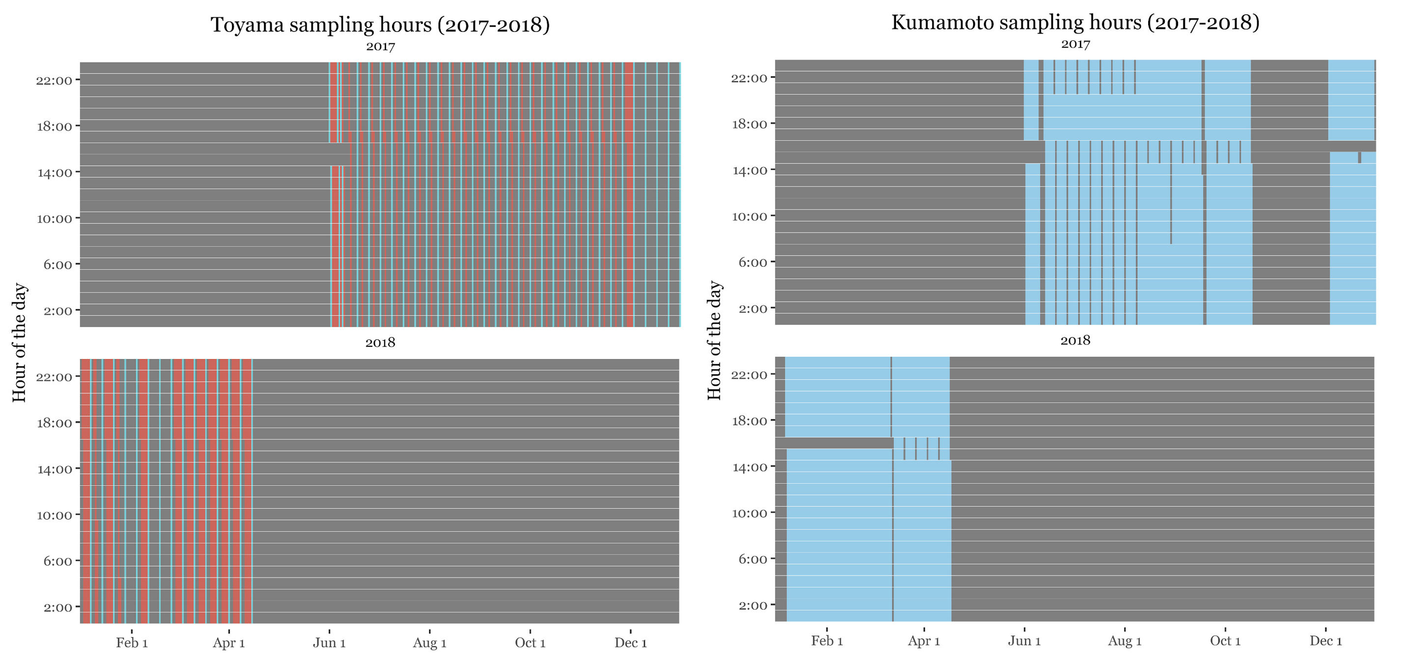
Hours of the day sampled
If we look at the hours of the day in which the samples were taken, we can see that the samples for Noto had a very short schedule, taking samples from 12 to 15 hours for all samples (including the weekly ones) except for the intensive campaign with subdaily samples in which most of the day was covered:
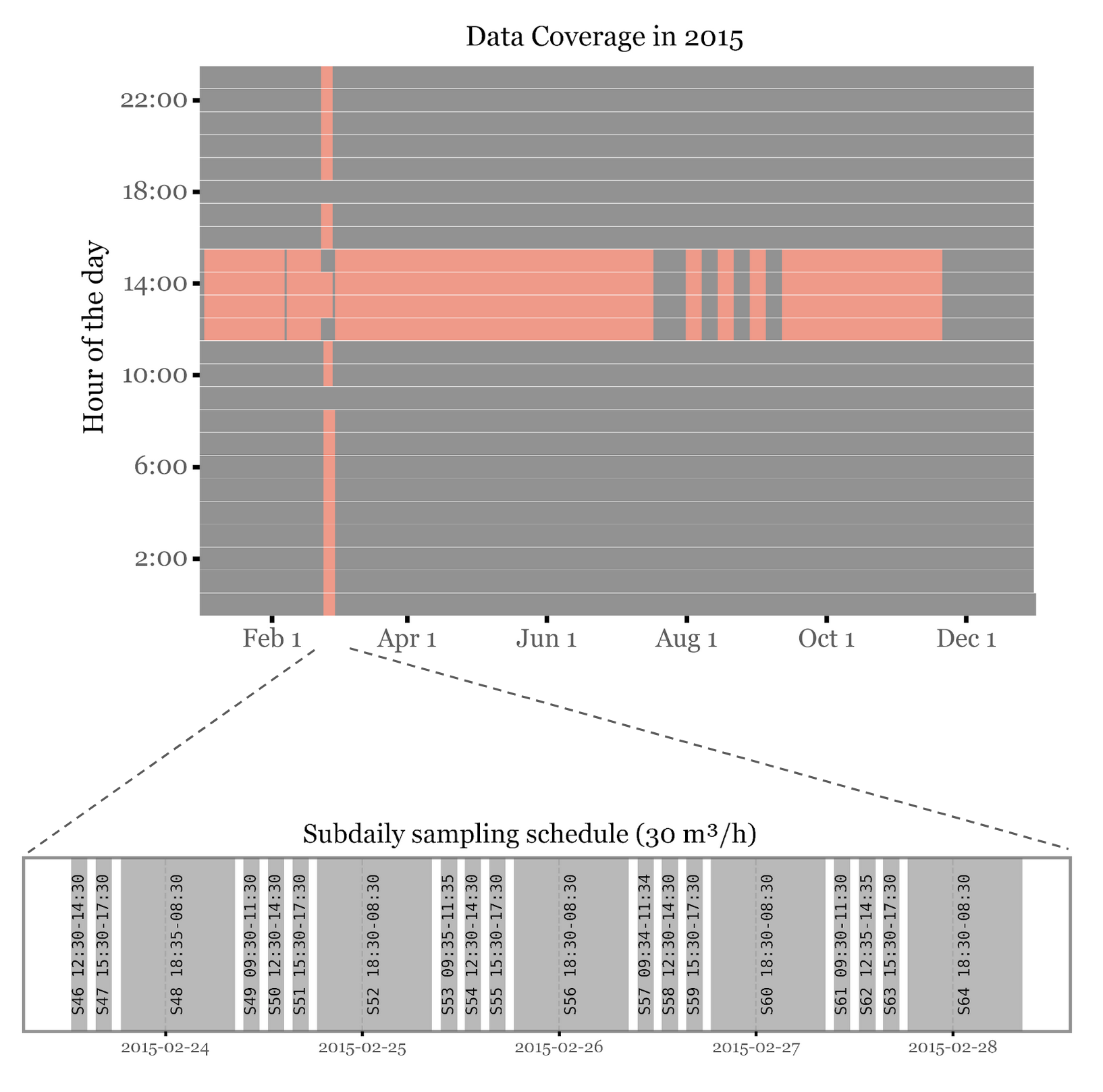
This is important because as seen in (Gusareva et al. 2019) showed, there is a diurnal pattern in the composition of the air microbiome, with different taxa being more abundant at different times of the day, so that if we want to have a complete coverage of the air microbiome we need to sample for the whole day.
For Kumamoto and Toyama, the samples now spanned for basically the whole day:
Analysis
Blanks vs Samples
Let’s take a preliminary look at some metrics for the “blanks” and how they compare to the samples (stratified by header type, just in case).
If we look at the diversity at the genus level, which is basically the number of different genera found in each sample:
clean_kumamoto.to_csv('../checkpoints/clean_kumamoto.csv', index=False)clean_kumamoto.query('rank=="Genus"').query('reads > 0').to_csv('../checkpoints/clean_kumamoto_genus.csv', index=False)clean_toyama.query('rank=="Genus"').query('reads > 0').to_csv('../checkpoints/clean_toyama_genus.csv', index=False)
clean_toyama.query('rank=="Species"').query('reads > 0').to_csv('../checkpoints/clean_toyama_species.csv', index=False)clean_toyama.to_csv('../checkpoints/clean_toyama.csv', index=False)Show Code
diversity_kumamoto = (clean_kumamoto
 .assign(sample_type=lambda dd: np.where(dd.sample_id.str.startswith('KS'), 'Sample (PM$_{2.5}$)', 'Blank'))
 .assign(Kingdom=lambda dd: np.where(dd.Superkingdom == "Bacteria", "Bacteria", dd['Kingdom']))
 .query('rank=="Genus"')
 .query('Kingdom.isin(["Bacteria", "Fungi"])')
 .query('reads > 0')
 .groupby(['sample_type', 'sample_id', 'Kingdom'])
 .agg({'Genus': 'count'})
 .reset_index()
 .assign(location='Kumamoto')
)

diversity_toyama = (clean_toyama
 .merge(samples_info[['sample_id', 'header']], how='left')
 .assign(sample_type=lambda dd: np.where(dd.sample_id.str.startswith('TS'), dd['header'], 'Blank'))
 .assign(Kingdom=lambda dd: np.where(dd.Superkingdom == "Bacteria", "Bacteria", dd['Kingdom']))
 .query('rank=="Genus"')
 .query('Kingdom.isin(["Bacteria", "Fungi"])')
 .query('reads > 0')
 .groupby(['sample_type', 'sample_id', 'Kingdom'])
 .agg({'Genus': 'count'})
 .reset_index()
 .assign(location='Toyama')
 .replace({'sample_type': {'PM10': 'Sample (PM$_{10}$)', 'PM2.5': 'Sample (PM$_{2.5}$)'}})

)

(pd.concat([diversity_kumamoto, diversity_toyama])
 .pipe(lambda dd: p9.ggplot(dd)
 + p9.aes('location', 'Genus'))
 + p9.facet_wrap('~ Kingdom', scales='free_y')
 + p9.geom_jitter(p9.aes(color='sample_type'),alpha=.5, size=1.5, stroke=0,
                  position=p9.position_jitterdodge(jitter_width=.1))
 + p9.geom_boxplot(p9.aes(fill='sample_type'), outlier_alpha=0, alpha=.5)
 + p9.scale_color_manual(['#ab2422', '#D3894C', '#435B97'])
 + p9.scale_fill_manual(['#ab2422', '#D3894C', '#435B97'])
 + p9.labs(x='', y='Genus diversity', fill='', color='')
 + p9.theme(figure_size=(6, 2.5), legend_position='top')
)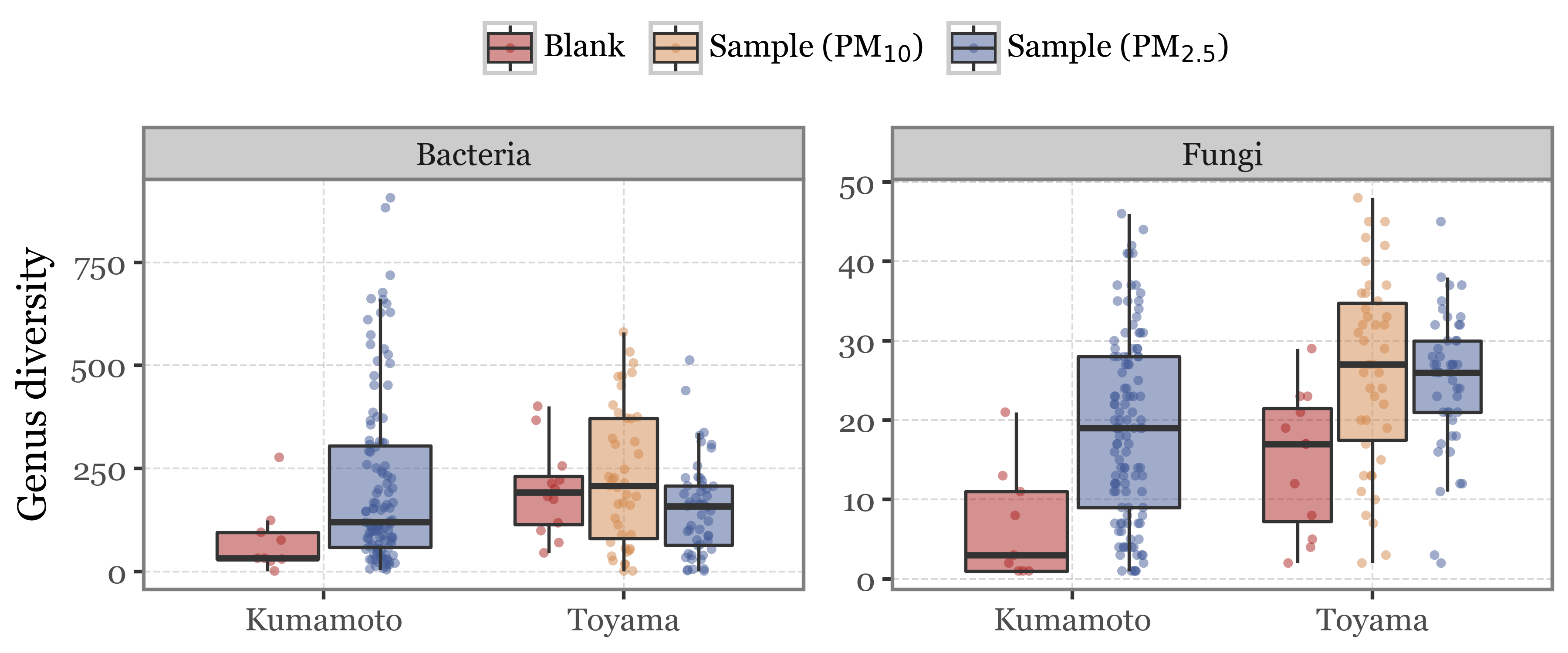
What we see is that the blanks have a comparable or even higher bacterial diversity than the samples in Toyama, but a lower bacterial diversity than Kumamoto. Some of the blanks still show a rather high diversity in Kumamoto too though.
Looking at the fungal diversity, both in Kumamoto and in Toyama the blanks have lower diversity than their respective samples, but the number of different Genera found in samples that should be “blanks” is still worryingly high…
Let’s now make the same comparison but for the number of reads per sample, which we somehow expect to be lower in blanks and is what we use (in part) to quantify the relative amount of each organism between samples:
Show Code
kingdom_bacteria_toyama = (clean_toyama
 .query('rank=="Superkingdom"')
 .query('Superkingdom=="Bacteria"')
 .assign(Kingdom='Bacteria')
 .assign(rank='Kingdom')
 .assign(location='Toyama')
 .merge(samples_info[['sample_id', 'header']], how='left')
 .assign(sample_type=lambda dd: np.where(dd.sample_id.str.startswith('TS'), dd['header'], 'Blank'))
 .replace({'sample_type': {'PM10': 'Sample (PM$_{10}$)', 'PM2.5': 'Sample (PM$_{2.5}$)'}})
)

kingdom_fungi_toyama = (clean_toyama
    .query('rank=="Kingdom"')
    .query('Kingdom=="Fungi"')
    .assign(location='Toyama')
    .merge(samples_info[['sample_id', 'header']], how='left')
    .assign(sample_type=lambda dd: np.where(dd.sample_id.str.startswith('TS'), dd['header'], 'Blank'))
    .replace({'sample_type': {'PM10': 'Sample (PM$_{10}$)', 'PM2.5': 'Sample (PM$_{2.5}$)'}})

    )

kingdom_bacteria_kumamoto = (clean_kumamoto
    .query('rank=="Superkingdom"')
    .query('Superkingdom=="Bacteria"')
    .assign(Kingdom='Bacteria')
    .assign(rank='Kingdom')
    .assign(location='Kumamoto')
     .assign(sample_type=lambda dd: np.where(dd.sample_id.str.startswith('KS'), 'Sample (PM$_{2.5}$)', 'Blank'))

    )
kingdom_fungi_kumamoto = (clean_kumamoto
    .query('rank=="Kingdom"')
    .query('Kingdom=="Fungi"')
    .assign(location='Kumamoto')
     .assign(sample_type=lambda dd: np.where(dd.sample_id.str.startswith('KS'), 'Sample (PM$_{2.5}$)', 'Blank'))

    )

(pd.concat([kingdom_bacteria_toyama, kingdom_fungi_toyama, kingdom_bacteria_kumamoto, kingdom_fungi_kumamoto])
  .groupby(['sample_type', 'sample_id', 'Kingdom', 'location'])
 .reads.sum()
 .reset_index()
  .pipe(lambda dd: p9.ggplot(dd)
 + p9.aes('location', 'reads')
 + p9.facet_wrap('~ Kingdom', scales='free_y')
 + p9.geom_boxplot(p9.aes(fill='sample_type'), outlier_alpha=0, alpha=.5)
 + p9.geom_jitter(p9.aes(color='sample_type'), alpha=.5, size=1.5, stroke=0,
                  position=p9.position_jitterdodge(jitter_width=.1))
 + p9.scale_color_manual(['#ab2422', '#D3894C', '#435B97'])
 + p9.scale_fill_manual(['#ab2422', '#D3894C', '#435B97'])
 + p9.labs(x='', y='Total Reads', fill='', color='')
 + p9.theme(figure_size=(6, 2.5), legend_position='top')
  )
)
The metrics here are even worse, with the average number of bacterial reads in blanks being higher than in samples in both sites. Numbers are better for fungi, which show a lower average number of reads in blanks, but the total amount is still significant for a blank that sampled a total of 0 m3 of air…
Now, the database we used also matches reads to organisms outside the kingdoms of Bacteria or Fungi: matches to the Homo sapiens species (and all of its higher level taxonomic clades) were also considered.
While the blanks are not sterile blanks, but rather a control for the normal handling of a filter without actually filtered air, one would expect human DNA to be more commonplace in the blanks with respect to the actual samples. We expect some circulating human DNA everywhere but the one (if any) introduced via the filter manipulation should be specially overrepresented in the blanks.
Lets then take a look at the number of reads assigned to Homo sapiens by sample type and location:
Show Code
human_kumamoto = (pd.concat([clean_kumamoto.query('rank=="Kingdom"'),
                             kingdom_bacteria_kumamoto.drop(columns=['location', 'sample_type'])])
    .groupby(['sample_id'])
    .apply(lambda dd: dd.assign(relative_abundance=(dd.reads / dd.reads.sum()).fillna(0)))
    .reset_index(drop=True)
    .query('Kingdom=="Metazoa"')
    .assign(location='Kumamoto')
     .assign(sample_type=lambda dd: np.where(dd.sample_id.str.startswith('KS'), 'Sample (PM$_{2.5}$)', 'Blank'))
    )


human_toyama = (pd.concat([clean_toyama.query('rank=="Kingdom"'),
                          kingdom_bacteria_toyama.drop(columns=['location', 'sample_type', 'header'])])
    .merge(samples_info[['sample_id', 'header']], how='left', on='sample_id')
    .groupby(['sample_id'])
    .apply(lambda dd: dd.assign(relative_abundance=(dd.reads / dd.reads.sum()).fillna(0)))
    .reset_index(drop=True)
    .query('Kingdom=="Metazoa"')
    .assign(location='Toyama')
    .assign(sample_type=lambda dd: np.where(dd.sample_id.str.startswith('TS'), dd['header'], 'Blank'))
    .replace({'sample_type': {'PM10': 'Sample (PM$_{10}$)', 'PM2.5': 'Sample (PM$_{2.5}$)'}})
    )

(pd.concat([human_kumamoto, human_toyama])
 .query('sample_type.notna()')
 .assign(relative_abundance=lambda dd: dd['relative_abundance'].fillna(0))
 .replace({'Metazoa': 'Homo sapiens'})
 .drop(columns=taxa + ['taxid', 'name', 'header', 'rank'])
 .melt(['sample_id', 'location', 'sample_type'])
 .replace({'variable': {'reads': 'Homo sapiens reads',
                        'relative_abundance': 'Relative abundance of Homo sapiens reads'}})
   .pipe(lambda dd: p9.ggplot(dd)
 + p9.aes('location', 'value'))
 + p9.facet_wrap('~ variable', scales='free_y')
 + p9.geom_jitter(p9.aes(color='sample_type'),alpha=.5, size=1.5, stroke=0,
                  position=p9.position_jitterdodge(jitter_width=.1))
 + p9.geom_boxplot(p9.aes(fill='sample_type'), outlier_alpha=0, alpha=.5)
 + p9.scale_color_manual(['#ab2422', '#D3894C', '#435B97'])
 + p9.scale_fill_manual(['#ab2422', '#D3894C', '#435B97'])
 + p9.labs(x='', y='Total Reads', fill='', color='')
 + p9.theme(figure_size=(6, 2.5), legend_position='top')
)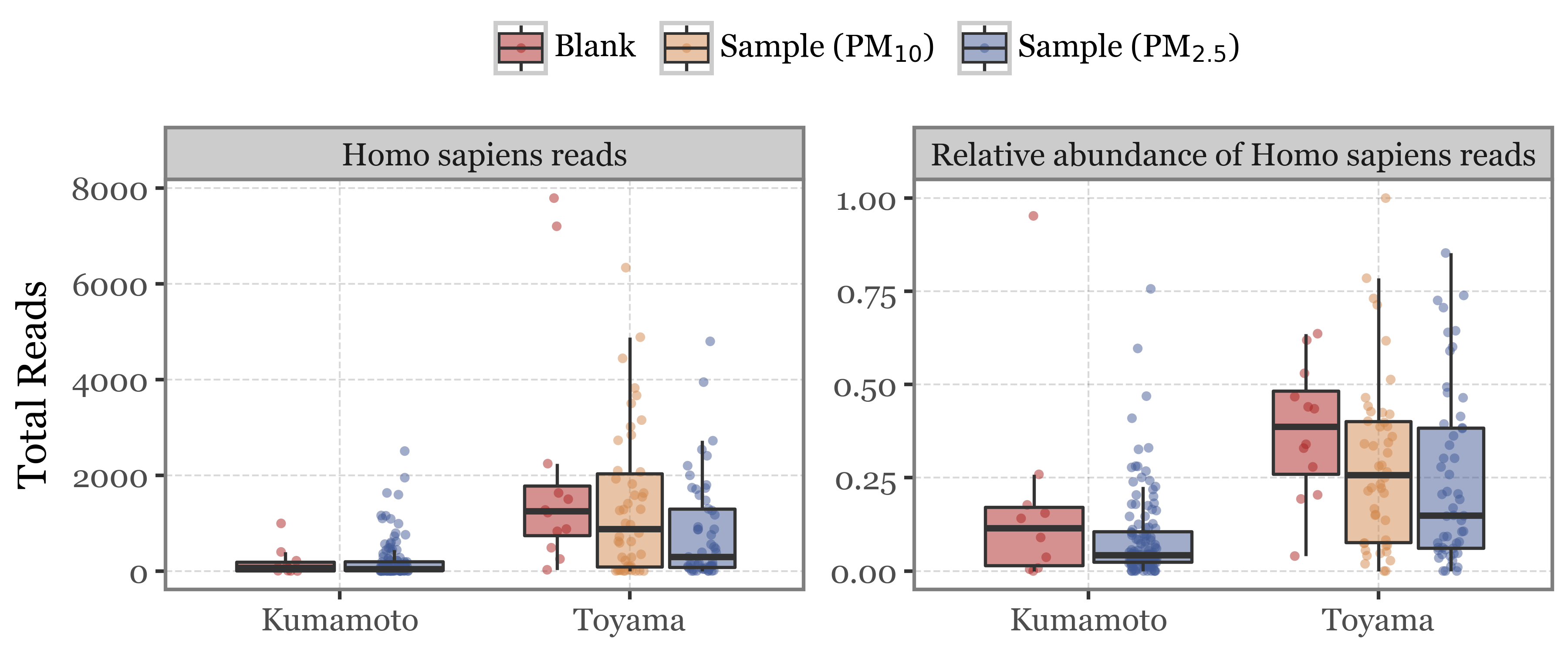
As we can see, first of all the total amount of human reads is way lower in Kumamoto than in Toyama, both in blanks and in samples. This could be an indication of either a cleaner/more sterile handling of the filters or simply an environment with less human activity/presence.
Human reads are also more common for both sites in the blanks rather than in the samples, which is to be expected.
Sequencing metrics evaluation
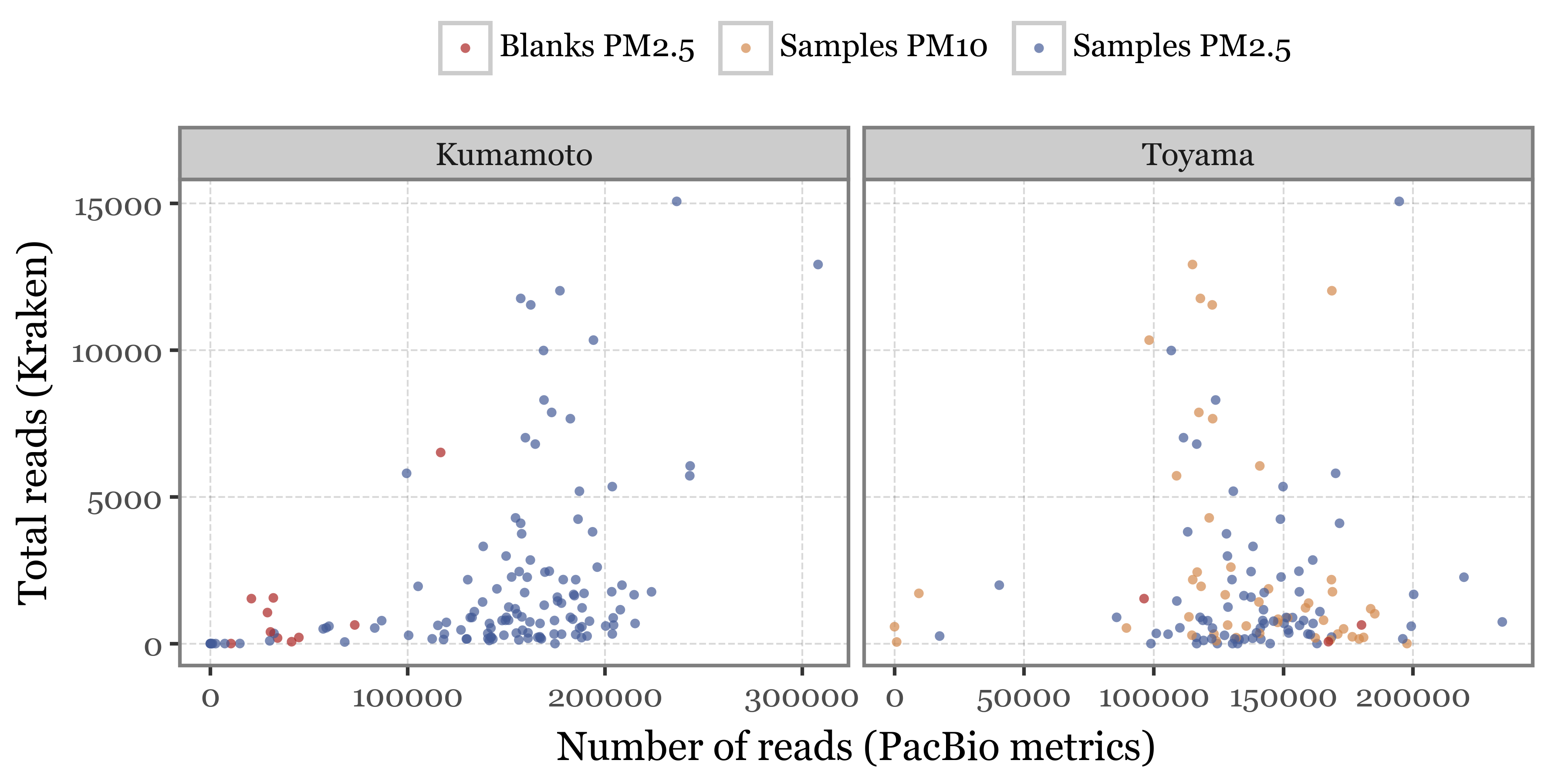
We have, however, another set of metrics we can use, which come directly from the sequencing report. We have the DNA yield, average read length, average read quality and number of reads.
I don’t know what is the difference between this “Number of reads” and the total number of reads that we can obtain directly from the Kraken output is, but the scale is really different, and the relationship between them is not really clear. See the comparison in the scatterplot below:
Code for pacbio metrics wrangling
pacbio_metrics = (pd.read_excel('../data/pacbio_samples_metrics.xlsx', sheet_name=1)
 .rename(columns={
     'Names': 'sample_id',
     'DNA (ng)': 'dna_total',
     'Number_of_reads': 'n_reads',
     'Total_bases': 'total_bases',
     'Median_read_length': 'rl_median',
     'Mean_read_quality': 'qc_mean'
 })
 [['sample_id', 'dna_total', 'n_reads', 'total_bases', 'rl_median', 'qc_mean']]
  .assign(header=lambda dd: np.where(dd.sample_id.str.endswith('.1'), 'PM10', 'PM2.5'))
  .assign(sample_id=lambda dd: np.where(dd.sample_id.str.startswith('T'), dd['sample_id'],
                                         dd['sample_id'].str[:2] + dd['sample_id'].str[2:].str.zfill(3)))
  .assign(sample_type=lambda dd: np.where(dd.sample_id.str.contains('B', regex=False), 'Blank', 'Sample'))
)

kumamoto_reads = (kumamoto_all
 .query('taxid==1')
 .melt(['lvl_type', 'taxid', 'name'])
 .query('not variable.isin(["#perc", "tot_all", "tot_lvl"])')
 .query('variable.str.contains("all")')
 .assign(variable=lambda dd: dd['variable'].str.split('_').str[0].map(kraken_to_sample_map_kumamoto))
 .assign(sample_type=lambda dd: np.where(dd['variable'].str.startswith('KS'), 'Sample', 'Blank'))
 .assign(value=lambda dd: dd['value'].astype(int))
 .assign(sample_id=lambda dd: dd.variable.str[:2] + dd.variable.str[2:].str.zfill(3))
 .rename(columns={'value': 'reads'})
 [['sample_id', 'reads']]
)

toyama_reads = (kumamoto_all
 .query('taxid==1')
 .melt(['lvl_type', 'taxid', 'name'])
 .query('not variable.isin(["#perc", "tot_all", "tot_lvl"])')
 .query('variable.str.contains("all")')
 .assign(variable=lambda dd: dd['variable'].str.split('_').str[0].map(kraken_to_sample_map_toyama))
 .assign(sample_type=lambda dd: np.where(dd['variable'].str.startswith('TS'), 'Sample', 'Blank'))
 .assign(value=lambda dd: dd['value'].astype(int))
 .assign(sample_id=lambda dd: dd.variable.str[:2] + dd.variable.str[2:].str.zfill(3).str.replace('_', '.'))
  .rename(columns={'value': 'reads'})
 [['sample_id', 'reads']]
)
Show Code
 (pacbio_metrics
 .merge(pd.concat([kumamoto_reads, toyama_reads]), how='left', on='sample_id')
 .assign(location=lambda dd: np.where(dd.sample_id.str.startswith('K'), 'Kumamoto', 'Toyama'))
 .dropna()
 # just removing the sample with 500k reads and 0 reads in Kraken for better visualization
 .query('n_reads < 500000')
 .assign(sample_label=lambda dd: dd.sample_type + 's ' + dd.header.fillna(''))
 .pipe(lambda dd: p9.ggplot(dd)
       + p9.aes('n_reads', 'reads')
       + p9.geom_point(p9.aes(color='sample_label'), stroke=0, alpha=.7)
       + p9.scale_color_manual(['#ab2422', '#D3894C', '#435B97'])
       + p9.facet_wrap('~ location', scales='free_x')
       + p9.labs(x='Number of reads (PacBio metrics)', y='Total reads (Kraken)', color='')
       + p9.theme(figure_size=(6, 3),
                  legend_position='top')
 )
)
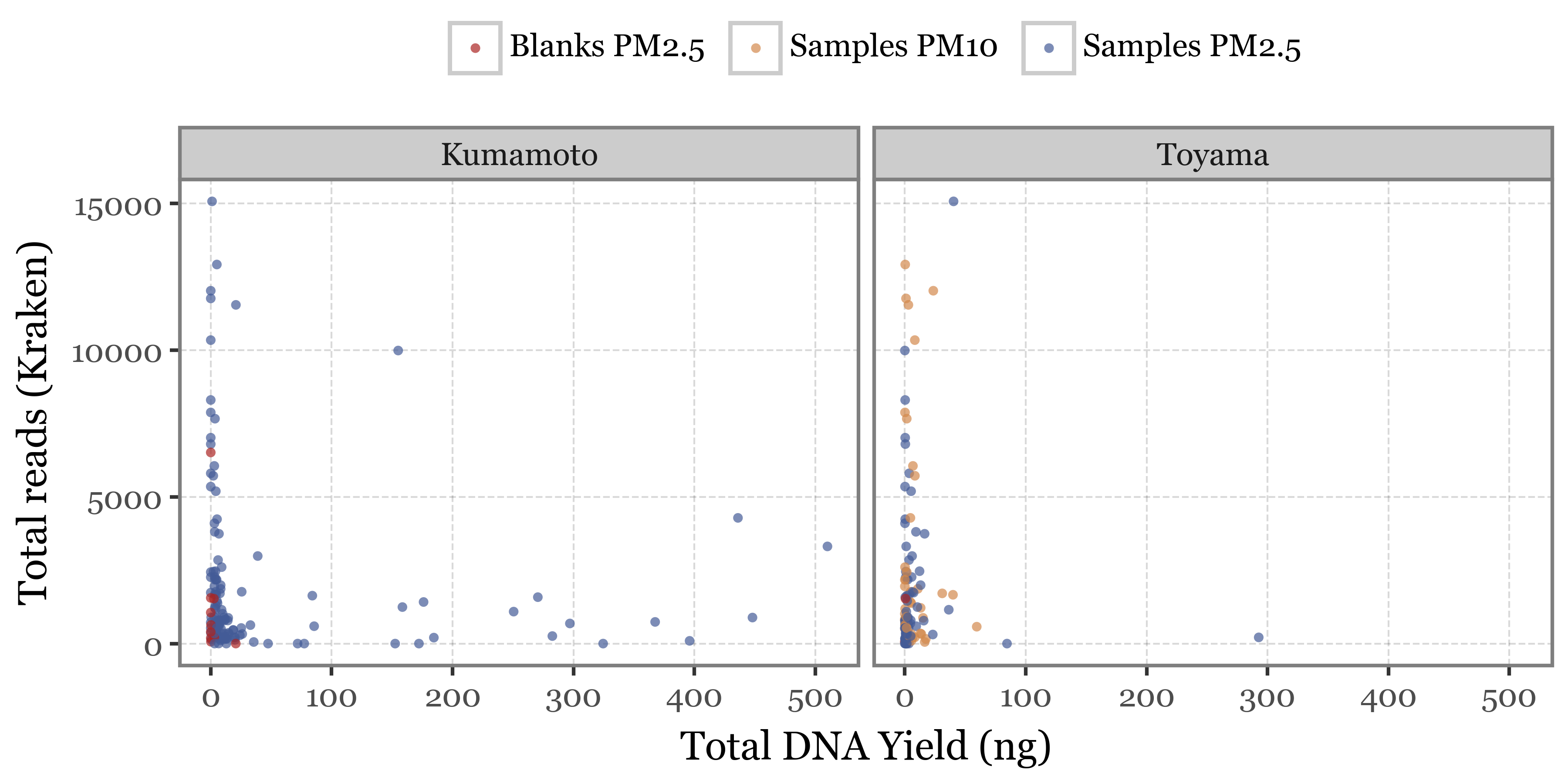
The relationship between DNA yield and number of reads is also not clear, while one would expect a higher DNA yield to be associated with a higher number of reads, if no other amplification steps were taken, yet that doesn’t seem to be the case for either the total number of reads we get from the PacBio stats nor the number of reads we get from the Kraken output, which is even more anticorrelated with the DNA yield:
Show Code
(pacbio_metrics
 .merge(pd.concat([kumamoto_reads, toyama_reads]), how='left', on='sample_id')
 .assign(location=lambda dd: np.where(dd.sample_id.str.startswith('K'), 'Kumamoto', 'Toyama'))
 .dropna()
 # just removing the sample with 500k reads and 0 reads in Kraken for better visualization
 .query('n_reads < 500000')
#  .query('dna_total < 100')
 .assign(sample_label=lambda dd: dd.sample_type + 's ' + dd.header.fillna(''))
 .pipe(lambda dd: p9.ggplot(dd)
       + p9.aes('dna_total', 'n_reads')
       + p9.geom_point(p9.aes(color='sample_label'), stroke=0, alpha=.7)
       + p9.scale_color_manual(['#ab2422', '#D3894C', '#435B97'])
       + p9.facet_wrap('~ location')
       + p9.labs(x='Total DNA Yield (ng)', y='Total reads (PacBio)', color='')
       + p9.theme(figure_size=(6, 3),
                  legend_position='top')
 )
)
Show Code
(pacbio_metrics
 .merge(pd.concat([kumamoto_reads, toyama_reads]), how='left', on='sample_id')
 .assign(location=lambda dd: np.where(dd.sample_id.str.startswith('K'), 'Kumamoto', 'Toyama'))
 .dropna()
 # just removing the sample with 500k reads and 0 reads in Kraken for better visualization
 .query('n_reads < 500000')
#  .query('dna_total < 100')
 .assign(sample_label=lambda dd: dd.sample_type + 's ' + dd.header.fillna(''))
 .pipe(lambda dd: p9.ggplot(dd)
       + p9.aes('dna_total', 'reads')
       + p9.geom_point(p9.aes(color='sample_label'), stroke=0, alpha=.7)
       + p9.scale_color_manual(['#ab2422', '#D3894C', '#435B97'])
       + p9.facet_wrap('~ location')
       + p9.labs(x='Total DNA Yield (ng)', y='Total reads (Kraken)', color='')
       + p9.theme(figure_size=(6, 3),
                  legend_position='top')
 )
)
In any case, it seems that the quality control metrics do not change much between blanks and samples, which is a good sign, but the total reads from the pacbio stats are definitely lower in blanks than in samples, which is also what we would expect if there is no contamination:
Show Code
(pacbio_metrics
 .assign(location=lambda dd: np.where(dd.sample_id.str.startswith('K'), 'Kumamoto', 'Toyama'))
 .merge(pd.concat([kumamoto_reads, toyama_reads]), how='left', on='sample_id')
 .melt(['sample_id', 'sample_type', 'header', 'location'],)
 .query('variable != "total_bases"')
 .query('variable != "dna_total"')
 .replace({'variable': {'dna_total': 'Total DNA (ng)', 'n_reads': 'Total reads (PacBio)',
                        'reads': 'Total reads (Kraken)',
                        'rl_median': 'Median read length',
                        'qc_mean': 'Average read quality'}})
 .assign(sample_label=lambda dd:  dd.sample_type + 's ' + dd.header.fillna(''))
 .pipe(lambda dd: p9.ggplot(dd) + p9.aes('location', 'value'))
    + p9.geom_jitter(p9.aes(color='sample_label', group='sample_label'), size=1.5, stroke=0, alpha=.5,
                     position=p9.position_jitterdodge(jitter_width=.1))
    + p9.facet_wrap('~ variable', scales='free_y')
    + p9.geom_boxplot(p9.aes(fill='sample_label'), outlier_alpha=0, alpha=.5)
    + p9.labs(x='', y='', fill='', color='')
    + p9.scale_color_manual(['#ab2422', '#D3894C', '#435B97'])
    + p9.scale_fill_manual(['#ab2422', '#D3894C', '#435B97'])
    + p9.theme(figure_size=(5, 3),
               axis_text_y=p9.element_text(size=7),
               legend_position='top')
   )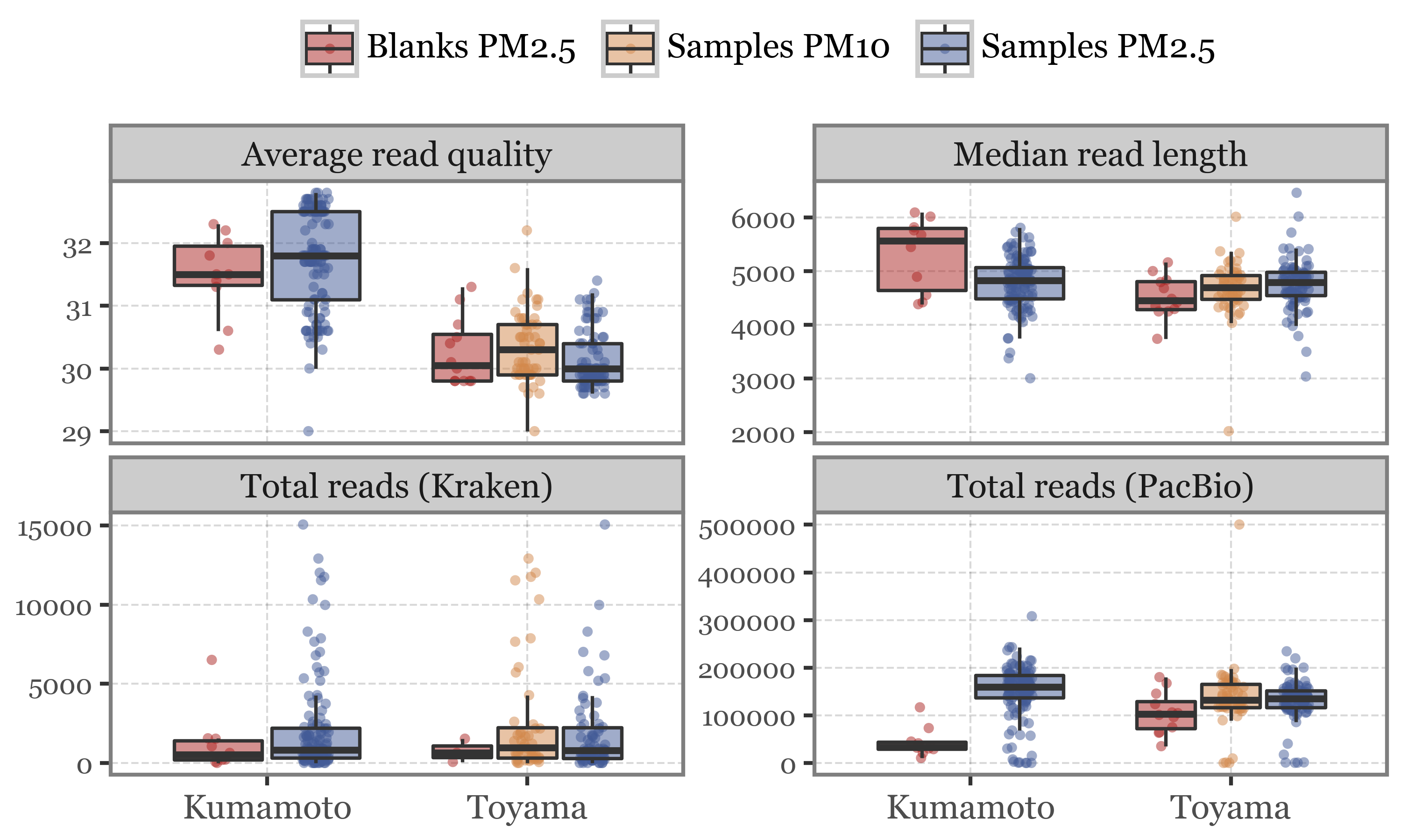
The odd case still is the number of reads from the Kraken output, which is in the same order of magnitude for blanks and samples, indicating some sort of error in the post-processing?
When looking at the DNA yield, the blanks are clearly lower than the samples, as we would expect for a sample that has not been exposed to air (or barely so).
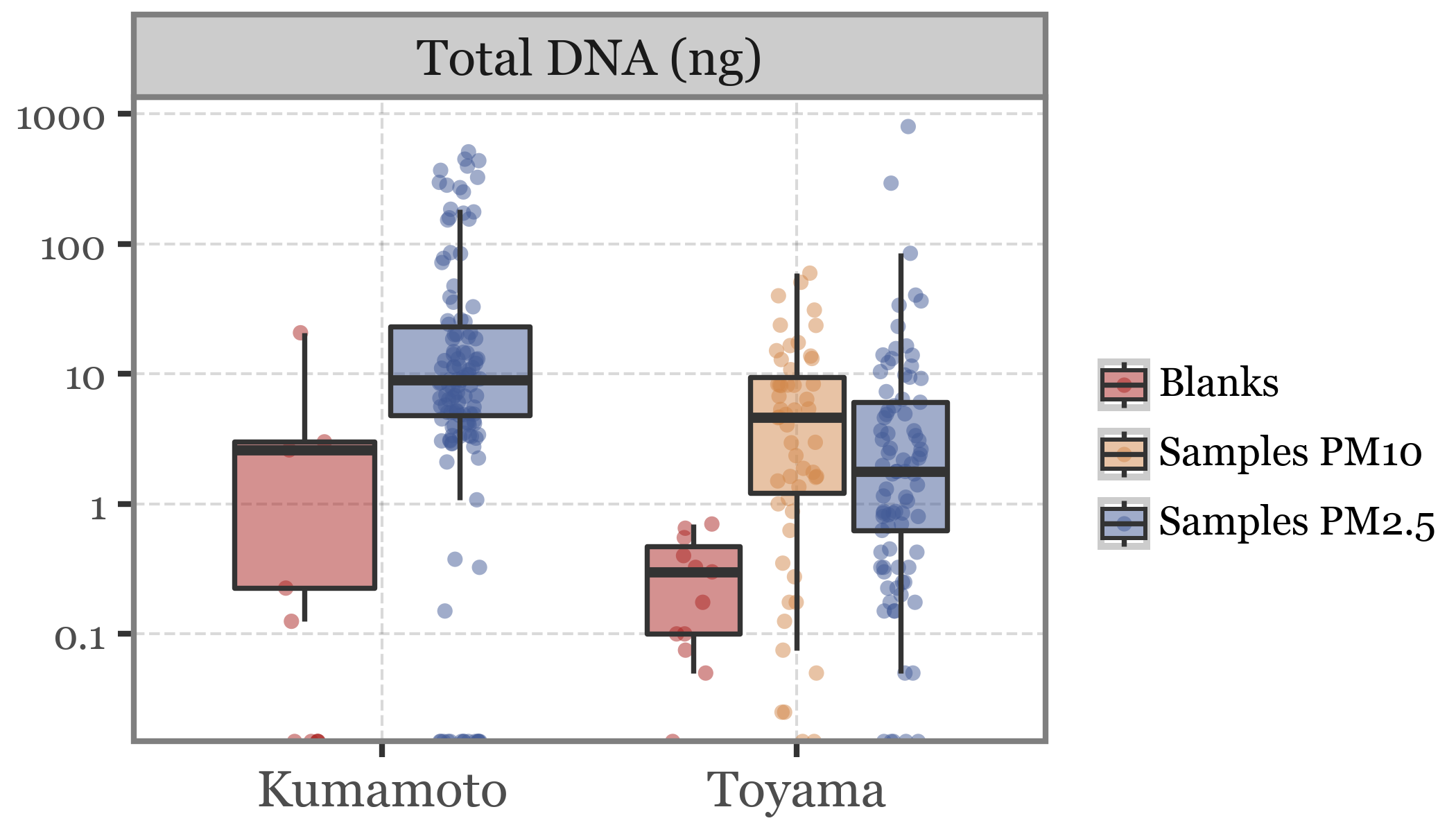
The few outliers in Total DNA make it quite difficult to actually see the differences between groups, so we will zoom into this variable and use a logarithmic scale to be able to visualize this:
Show Code
(pacbio_metrics
 .assign(location=lambda dd: np.where(dd.sample_id.str.startswith('K'), 'Kumamoto', 'Toyama'))
 .melt(['sample_id', 'sample_type', 'header', 'location'],)
 .query('variable != "total_bases"')
 .query('variable=="dna_total"')
 .replace({'variable': {'dna_total': 'Total DNA (ng)', 'n_reads': 'Number of reads', 'rl_median': 'Median read length',
                        'qc_mean': 'Average read quality'}})
 .assign(sample_label=lambda dd:  dd.sample_type + 's ' + dd.header.fillna(''))
 .replace({'Blanks PM2.5': 'Blanks'})
 .pipe(lambda dd: p9.ggplot(dd) + p9.aes('location', 'value'))
    + p9.geom_jitter(p9.aes(color='sample_label', group='sample_label'), size=1.5, stroke=0, alpha=.5,
                     position=p9.position_jitterdodge(jitter_width=.1))
    + p9.facet_wrap('~ variable', scales='free_y')
    + p9.geom_boxplot(p9.aes(fill='sample_label'), outlier_alpha=0, alpha=.5)
    + p9.labs(x='', y='', fill='', color='')
    + p9.scale_color_manual(['#ab2422', '#D3894C', '#435B97'])
    + p9.scale_fill_manual(['#ab2422', '#D3894C', '#435B97'])
    + p9.scale_y_continuous(trans='log10')
    + p9.theme(figure_size=(3.5, 2),
               axis_text_y=p9.element_text(size=7),
               legend_key_size=10,
               legend_text=p9.element_text(size=7),
               legend_position='right')
   )
Show Code
(pacbio_metrics
 .assign(location=lambda dd: np.where(dd.sample_id.str.startswith('K'), 'Kumamoto', 'Toyama'))
 .melt(['sample_id', 'sample_type', 'header', 'location'],)
 .query('variable != "total_bases"')
 .query('variable=="dna_total"')
 .replace({'variable': {'dna_total': 'Total DNA (ng)', 'n_reads': 'Number of reads', 'rl_median': 'Median read length',
                        'qc_mean': 'Average read quality'}})
 .assign(sample_label=lambda dd:  dd.sample_type + 's ' + dd.header.fillna(''))
 .replace({'Blanks PM2.5': 'Blanks'})
 .query('value < 100')
 .pipe(lambda dd: p9.ggplot(dd) + p9.aes('location', 'value'))
    + p9.geom_jitter(p9.aes(color='sample_label', group='sample_label'), size=1.5, stroke=0, alpha=.5,
                     position=p9.position_jitterdodge(jitter_width=.1))
    + p9.facet_wrap('~ variable', scales='free_y')
    + p9.geom_boxplot(p9.aes(fill='sample_label'), outlier_alpha=0, alpha=.5)
    + p9.labs(x='', y='', fill='', color='')
    + p9.scale_color_manual(['#ab2422', '#D3894C', '#435B97'])
    + p9.scale_fill_manual(['#ab2422', '#D3894C', '#435B97'])
    + p9.theme(figure_size=(3.5, 2),
               axis_text_y=p9.element_text(size=7),
               legend_key_size=10,
               legend_text=p9.element_text(size=7),
               legend_position='right')
   )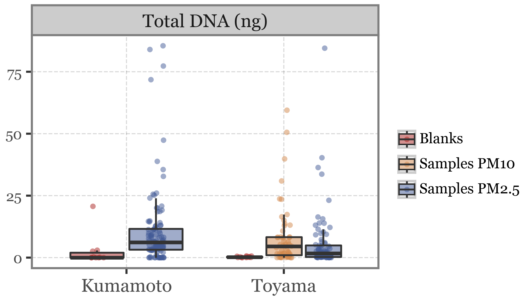
The differences in DNA yield seems to be somewhat proportional to the volume of air filtered, which makes sense if we assume that the DNA accumulates without issues in the filter.
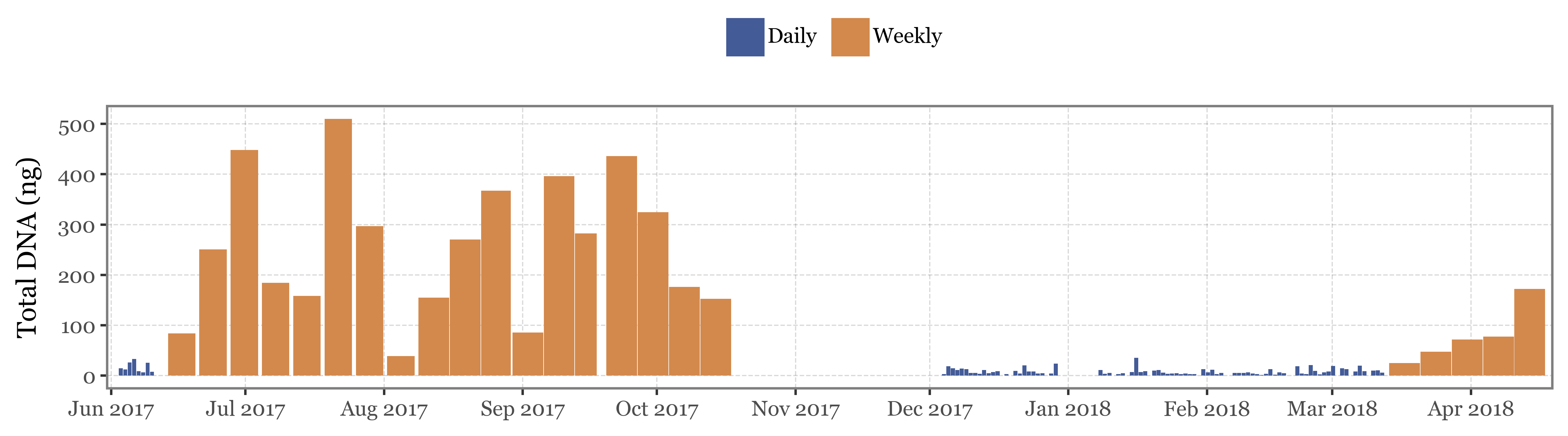
If we show the DNA yield by sample/date for Kumamoto, the samples with the higher yield are those which were sampling for the longest time:
Show Code
(pacbio_metrics
 .query('sample_id.str.startswith("K")')
 .assign(sample_type=lambda dd: np.where(dd.sample_id.str.contains('B'), 'Blank', 'Sample'))
 .merge(kumamoto_samples)
.assign(center_date=lambda dd: dd.start_dt + pd.to_timedelta(dd.duration / 2, unit='h'))
.assign(duration_name=lambda dd: np.where(dd.duration < 30, 'Daily', 'Weekly'))
 .pipe(lambda dd: p9.ggplot(dd)
         + p9.aes(x='center_date', y='dna_total')
       + p9.geom_col(p9.aes(fill='duration_name', x='center_date', width='duration / 24'))
       + p9.labs(x='', y='Total DNA (ng)', fill='')
       + p9.scale_fill_manual(['#435B97', '#D3894C'])
       + p9.scale_x_datetime(expand=(.005,  0, .005, 0), date_breaks='1 month', date_labels='%b %Y')

       + p9.theme(
           figure_size=(9, 2.5),
           legend_position='top',
)
 )
)
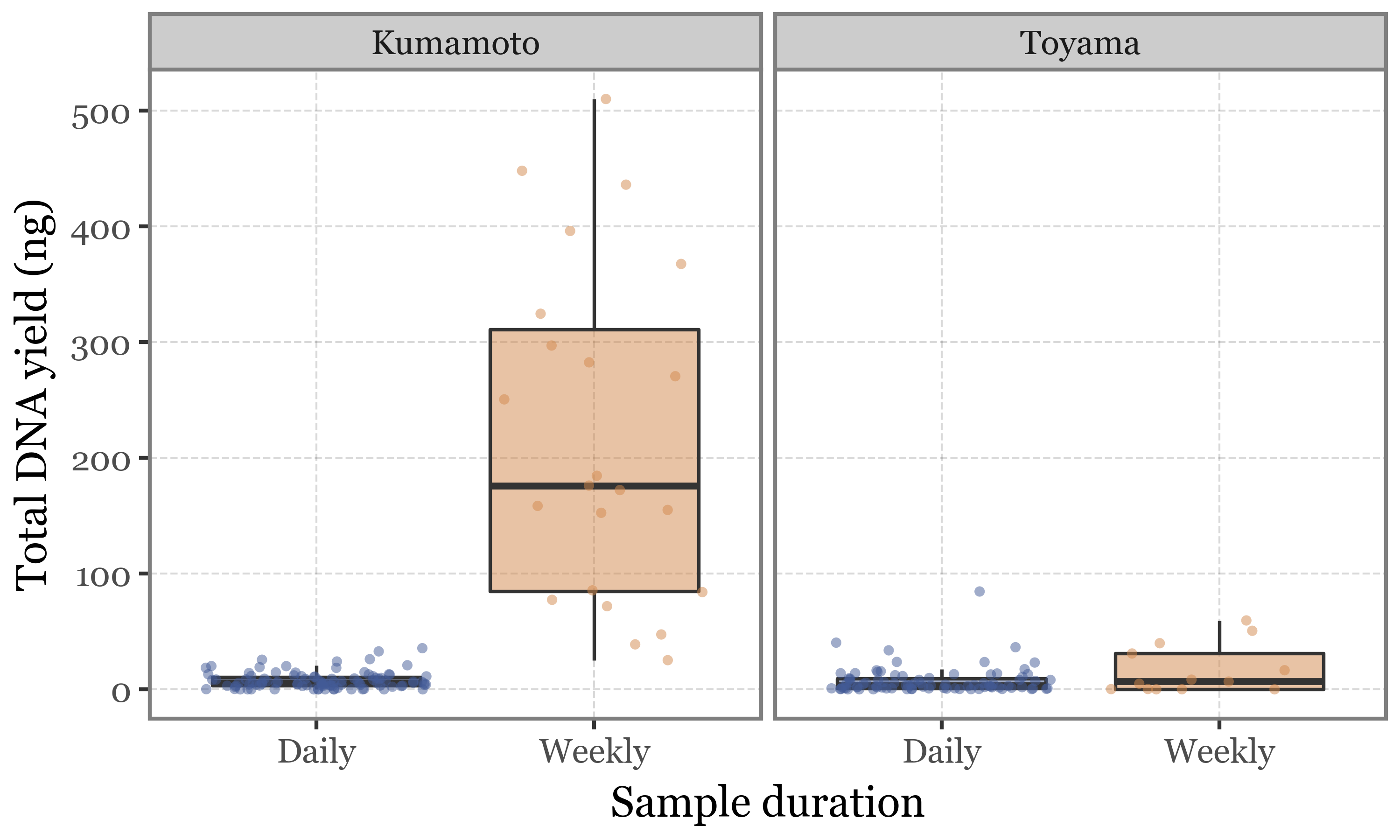
This would seem to be the expected behaviour, but this is not the case for Toyama, where daily and weekly samples have comparable DNA yields, completely independent of the volume of air filtered:
Show Code
(pacbio_metrics
 .assign(sample_id=lambda dd: dd.sample_id.str.replace('.1', '', regex=False))
 .merge(pd.concat([samples_info, kumamoto_samples]), how='left', on='sample_id')
 .dropna()
 .assign(duration_name=lambda dd: np.where(dd.duration < 30, 'Daily', 'Weekly'))
 .assign(location=lambda dd: np.where(dd.sample_id.str.startswith('K'), 'Kumamoto', 'Toyama'))
 .pipe(lambda dd: p9.ggplot(dd)
       + p9.aes('duration_name', 'dna_total')
       + p9.geom_boxplot(p9.aes(fill='duration_name'), outlier_alpha=0, alpha=.5)
       + p9.geom_jitter(p9.aes(color='duration_name'), alpha=.5, size=1.5, stroke=0)
       + p9.scale_color_manual(['#435B97', '#D3894C'])
       + p9.scale_fill_manual(['#435B97', '#D3894C'])
       + p9.facet_wrap('~ location')
       + p9.guides(fill=False, color=False)
       + p9.theme(figure_size=(5, 3),
                  legend_position='top')
       + p9.labs(x='Sample duration', y='Total DNA yield (ng)', fill='', color='')
 )
)
But even if we correct by the total volume of air filtered, the DNA yield is still higher in the longer (weekly) samples than in the shorter daily ones in Kumamoto, and a bit lower in the longer samples in Toyama, which is kind of expected if we consider the possible degradation/damage of the DNA in the filter after a longer exposure:
Show Code
(pacbio_metrics
 .assign(sample_id=lambda dd: dd.sample_id.str.replace('.1', '', regex=False))
 .merge(pd.concat([samples_info, kumamoto_samples]).drop(columns='header'), how='left', on='sample_id')
 .dropna()
 .assign(duration_name=lambda dd: np.where(dd.duration < 30, 'Daily', 'Weekly'))
 .assign(location=lambda dd: np.where(dd.sample_id.str.startswith('K'), 'Kumamoto', 'Toyama'))
 .assign(label=lambda dd: dd['duration_name'] + '\n(' + dd['header'] + ')')
 .pipe(lambda dd: p9.ggplot(dd)
       + p9.aes('label', 'dna_total / volume')
       + p9.geom_boxplot(p9.aes(fill='duration_name'), outlier_alpha=0, alpha=.5)
       + p9.geom_jitter(p9.aes(color='duration_name'), alpha=.5, size=1.5, stroke=0)
       + p9.scale_color_manual(['#435B97', '#D3894C'])
       + p9.scale_fill_manual(['#435B97', '#D3894C'])
       + p9.facet_wrap('~ location', scales='free_x')
       + p9.guides(fill=False, color=False)
       + p9.theme(figure_size=(5, 2.5),
                  legend_position='top')
       + p9.labs(x='', y='Total DNA (ng/m3)', fill='', color='')
 )
)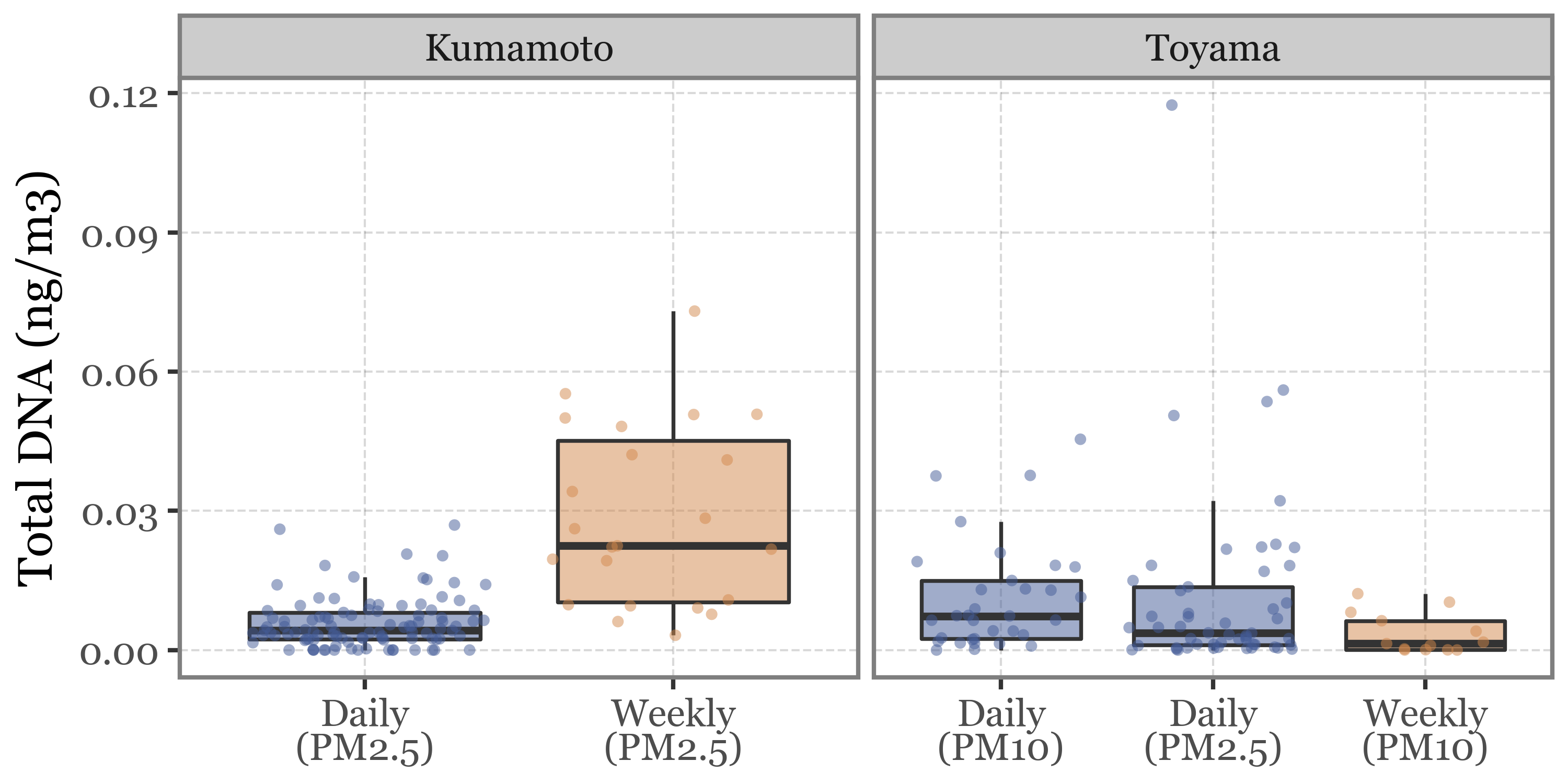
What might be the explanation? Weekly samples in Toyama use a different header (PM10 instead of PM2.5 in Kumamoto), but is this enough of a difference to explain the discrepancy?
What happens if we look at the total read counts by sample duration and header then? Wonder no more:
Show Code
all_reads = pd.concat([kumamoto_reads,
                       toyama_reads.assign(sample_id=lambda dd: dd.sample_id.str.replace('.1', '', regex=False))])

(pacbio_metrics
 .assign(sample_id=lambda dd: dd.sample_id.str.replace('.1', '', regex=False))
 .merge(pd.concat([samples_info, kumamoto_samples]).drop(columns='header'), how='left', on='sample_id')
 .dropna()
 .assign(duration_name=lambda dd: np.where(dd.duration < 30, 'Daily', 'Weekly'))
 .assign(location=lambda dd: np.where(dd.sample_id.str.startswith('K'), 'Kumamoto', 'Toyama'))
 .assign(label=lambda dd: dd['duration_name'] + '\n(' + dd['header'] + ')')
 .merge(all_reads)
 .pipe(lambda dd: p9.ggplot(dd)
       + p9.aes('label', 'reads')
       + p9.geom_boxplot(p9.aes(fill='duration_name'), outlier_alpha=0, alpha=.5)
       + p9.geom_jitter(p9.aes(color='duration_name'), alpha=.5, size=1.5, stroke=0)
       + p9.scale_color_manual(['#435B97', '#D3894C'])
       + p9.scale_fill_manual(['#435B97', '#D3894C'])
       + p9.facet_wrap('~ location', scales='free_x')
       + p9.guides(fill=False, color=False)
       + p9.theme(figure_size=(5, 2.5),
                  legend_position='top')
       + p9.labs(x='', y='Total Kraken assigned reads', fill='', color='')
 )
)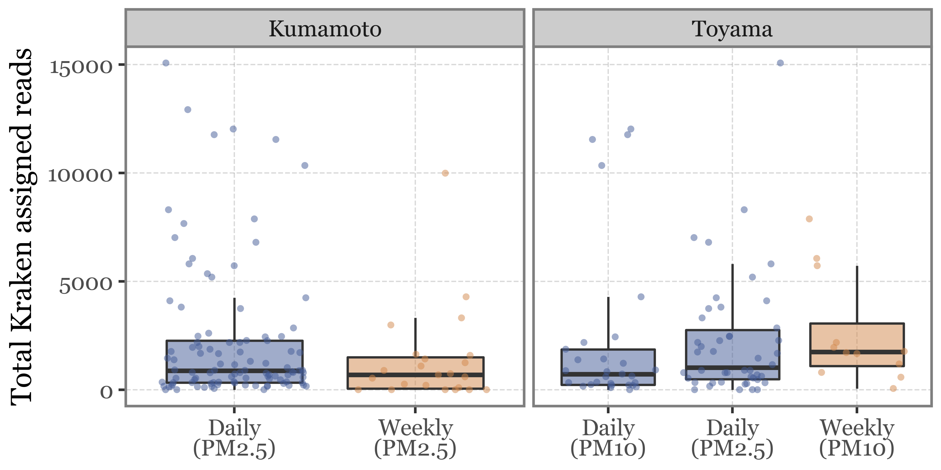
How come the total number of reads is always in the same range for all sample types given that the DNA yield is so different? If the number of reads was a proper measure of the amount of DNA (and by proxy, the biomass in the air) in the sample, we would expect a higher number of reads in the longer samples, but this is not the case.
Taxonomic Composition
Kumamoto
The composition of the samples at the high taxonomic level is rather variable, and specially if we were to use the total reads as a proxy of actual abundance:
Show Code
kumamoto_kingdoms = (pd.concat([clean_kumamoto.query('rank.isin(["Kingdom"])'),
           kingdom_bacteria_kumamoto])
 .query('Superkingdom != "Viruses"')
 .query('Superkingdom != "Archaea"')
 .merge(kumamoto_samples)
 .query('rank=="Kingdom"')
 .query('sample_id <= "KS120"')
 .groupby(['sample_id'])
 .apply(lambda dd: dd.assign(relative_abundance=(dd.reads / dd.reads.sum()).fillna(0)))
 .replace({'Kingdom': {'Metazoa': 'Human DNA', 'Viridiplantae': 'Green Plants'}}))

(kumamoto_kingdoms
 .pipe(lambda dd: p9.ggplot(dd) + p9.aes(x='sample_id', y='reads')
       + p9.geom_col(p9.aes(fill='Kingdom'))
       + p9.scale_y_continuous(expand=(.01, 0, .01, 0))
       + p9.scale_fill_manual(['#ab2422', '#D3894C', '#32a86d', '#435B97'])
       + p9.scale_x_discrete(breaks=sorted(dd.sample_id.unique())[::2])
       + p9.labs(x='', y='Total Reads', fill='')
       + p9.theme(
           axis_text_x=p9.element_text(angle=90, size=8, family='monospace'),
           legend_position='top',
           figure_size=(8, 2.5)
       )
       )
)
Show Code
(kumamoto_kingdoms
 .pipe(lambda dd: p9.ggplot(dd)
       + p9.aes(x='sample_id', y='relative_abundance')
       + p9.geom_col(p9.aes(fill='Kingdom'))
       + p9.scale_y_continuous(expand=(.0, 0, .0, 0), labels=percent_format())
       + p9.scale_fill_manual(['#ab2422', '#D3894C', '#32a86d', '#435B97'])
       + p9.scale_x_discrete(breaks=sorted(dd.sample_id.unique())[::2])
       + p9.labs(x='', y='Relative Abundance', fill='')
       + p9.guides(fill=False)
       + p9.theme(
           axis_text_x=p9.element_text(angle=90, size=8, family='monospace'),
           legend_position='top',
           figure_size=(8, 2),
           panel_background=p9.element_rect(fill='gray'),
           panel_grid=p9.element_blank()
       )
       )
)
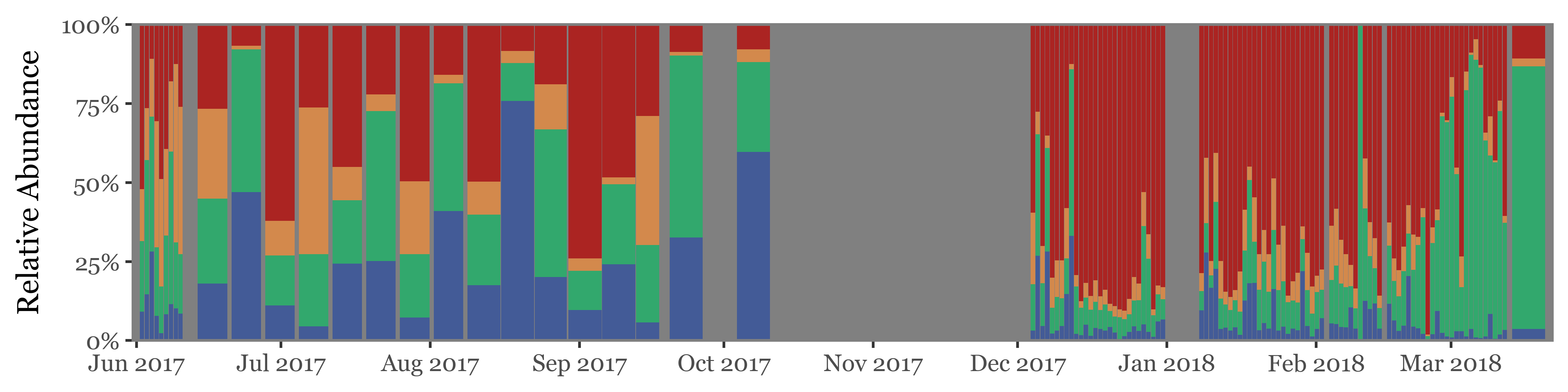
If instead of going sample by sample we use the actual timeline of the sampling, the total volume / time spent sampling for each sample becomes more evident. The fact that the total amount of reads for weekly samples, which have sampled 7 times the volume of the daily ones isn’t higher makes quite the case for NOT using total reads as a proxy for actual abundance in the enviroment/air:
Show Code
(kumamoto_kingdoms
 .assign(center_date=lambda dd: dd.start_dt + pd.to_timedelta(dd.duration / 2, unit='h'))
 .pipe(lambda dd: p9.ggplot(dd) + p9.aes(x='sample_id', y='reads')
       + p9.geom_col(p9.aes(fill='Kingdom', x='center_date', width='duration / 24'))
       + p9.scale_y_continuous(expand=(.01, 0, .01, 0))
       + p9.scale_fill_manual(['#ab2422', '#D3894C', '#32a86d', '#435B97'])
       + p9.scale_x_datetime(expand=(.005,  0, .005, 0), date_breaks='1 month', date_labels='%b %Y')
       + p9.labs(x='', y='Total Reads', fill='')
       + p9.guides(fill=False)
       + p9.theme(
           legend_position='top',
           figure_size=(8, 2),
       )
       )
)
Show Code
(kumamoto_kingdoms
 .assign(center_date=lambda dd: dd.start_dt + pd.to_timedelta(dd.duration / 2, unit='h'))
 .pipe(lambda dd: p9.ggplot(dd) + p9.aes(x='sample_id', y='relative_abundance')
       + p9.geom_col(p9.aes(fill='Kingdom', x='center_date', width='duration / 24'))
       + p9.scale_y_continuous(expand=(.0, 0, .0, 0), labels=percent_format())
       + p9.scale_fill_manual(['#ab2422', '#D3894C', '#32a86d', '#435B97'])
       + p9.scale_x_datetime(expand=(.005,  0, .005, 0), date_breaks='1 month', date_labels='%b %Y')
       + p9.labs(x='', y='Relative Abundance', fill='')
       + p9.guides(fill=False)
       + p9.theme(
           legend_position='top',
           figure_size=(8, 2),
           panel_background=p9.element_rect(fill='gray'),
           panel_grid=p9.element_blank()
       )
       )
)
Genus level
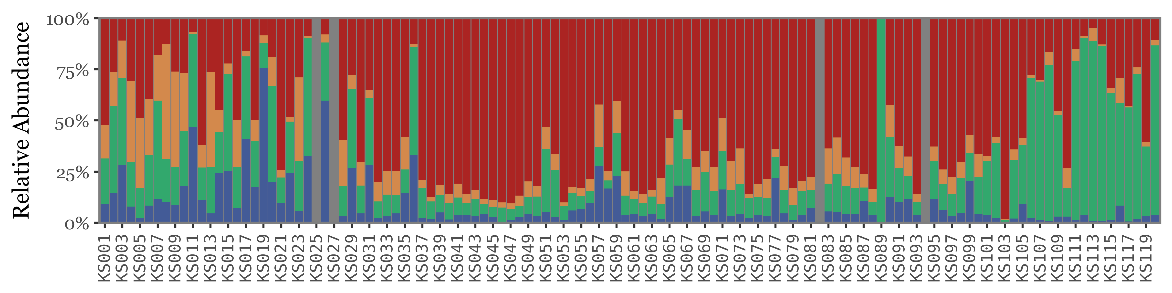
Let’s now go down to the genus level and explore the composition of the samples at this level. We are going to focus on fungi/bacteria now. We will represent the top 20 bacterial and fungal genera by their average relative abundance in the samples and group the rest of the genera in an “Other” category (representing 20 different colors is already a challenge, trying to show even more would be impossible).
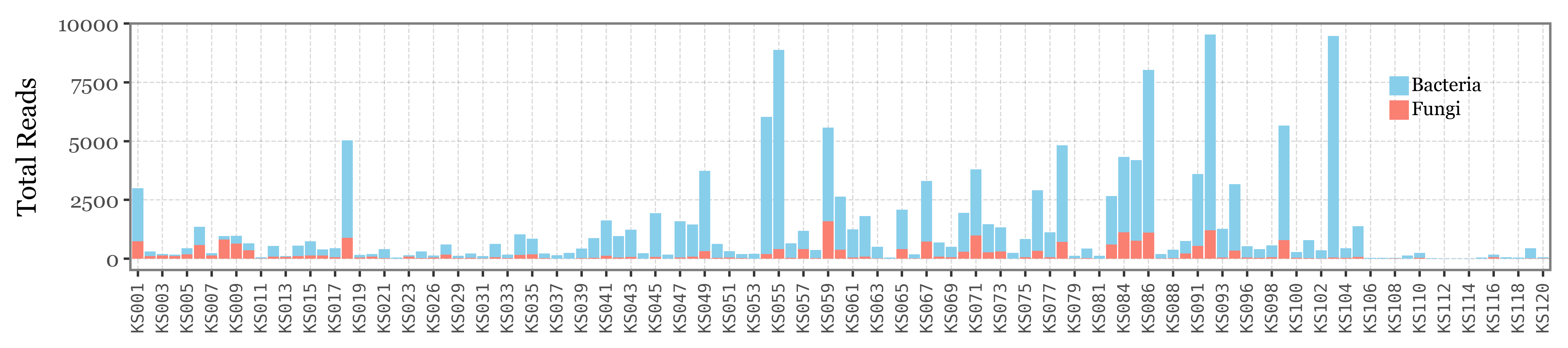
Let’s put the relative abundance values into context by showing the total reads assigned to either Bacteria (blue) or Fungi (red) in each sample, since there is a huge variability on a sample by sample basis:
Code for data wrangling of Genera
kumamoto_genera = (clean_kumamoto
.merge(kumamoto_samples)
.query('sample_id.str.startswith("KS")')
 .assign(Kingdom=lambda dd: np.where(dd.Superkingdom == 'Bacteria', 'Bacteria', dd.Kingdom))
 .query('Superkingdom != "Viruses"')
 .query('Superkingdom != "Archaea"')
 .query('Kingdom.isin(["Bacteria", "Fungi"])')
 .query('rank=="Genus"')
 .groupby(['sample_id', 'Kingdom'], as_index=False)
 .apply(lambda dd: dd.assign(relative_abundance=dd.reads / dd.reads.sum()))
 .drop(columns=['Species'])
)

top_genera = (kumamoto_genera
.groupby(['Kingdom', 'Genus'])
.agg({'relative_abundance': 'mean', 'reads': 'sum'})
.groupby('Kingdom', group_keys=False)
.apply(lambda dd: dd.nlargest(20, 'relative_abundance'))
.reset_index()
)

discrete_colors = [
    '#DB5F57', '#DB8657', '#DBAE57', '#DBD657', '#B9DB57', '#91DB57', '#69DB57', '#57DB6C',
    '#57DB94', '#57DBBB', '#57D3DB', '#57ACDB', '#5784DB', '#575CDB', '#7957DB', '#A157DB',
    '#C957DB', '#DB57C6', '#DB579E', '#DB5777', 'gray',
]
Show Code
(kumamoto_genera
 .groupby(['sample_id', 'Kingdom'])
 ['reads']
 .sum()
 .reset_index()
 .query('reads > 0')
 .pipe(lambda dd: p9.ggplot(dd)
  + p9.aes(x='sample_id', y='reads', fill='Kingdom')
  + p9.geom_col()
  + p9.scale_fill_manual(['skyblue', 'salmon'])
  + p9.scale_x_discrete(breaks=sorted(dd.sample_id.unique())[::2])
  + p9.labs(x='', y='Total Reads', fill='')
  + p9.theme(figure_size=(9, 2),
            legend_key_size=8,
            legend_position=(.95, .9),
            legend_text=p9.element_text(size=8),
            legend_title=p9.element_text(ha='center'),
            plot_title=p9.element_text(ha='center', family='Merriweather'),
            axis_text_x=p9.element_text(angle=90, size=7, family='monospace'),
 )
 )
)
Show Code
(kumamoto_genera
 .groupby(['sample_id', 'Kingdom'])
 ['reads']
 .sum()
 .reset_index()
 .query('reads > 0')
 .groupby('sample_id')
 .apply(lambda dd: dd.assign(relative_abundance=dd.reads / dd.reads.sum()))
 .pipe(lambda dd: p9.ggplot(dd)
  + p9.aes(x='sample_id', y='relative_abundance', fill='Kingdom')
  + p9.geom_col()
  + p9.scale_fill_manual(['skyblue', 'salmon'])
  + p9.scale_x_discrete(breaks=sorted(dd.sample_id.unique())[::2])
  + p9.scale_y_continuous(labels=percent_format(), expand=(.0, 0, .0, 0))
  + p9.labs(x='', y='Relative Abundance', fill='')
  + p9.theme(figure_size=(9, 2.25),
            legend_key_size=8,
            legend_position='top',
            legend_text=p9.element_text(size=8),
            legend_title=p9.element_text(ha='center'),
            plot_title=p9.element_text(ha='center', family='Merriweather'),
            axis_text_x=p9.element_text(angle=90, size=7, family='monospace'),
 )
 )
)
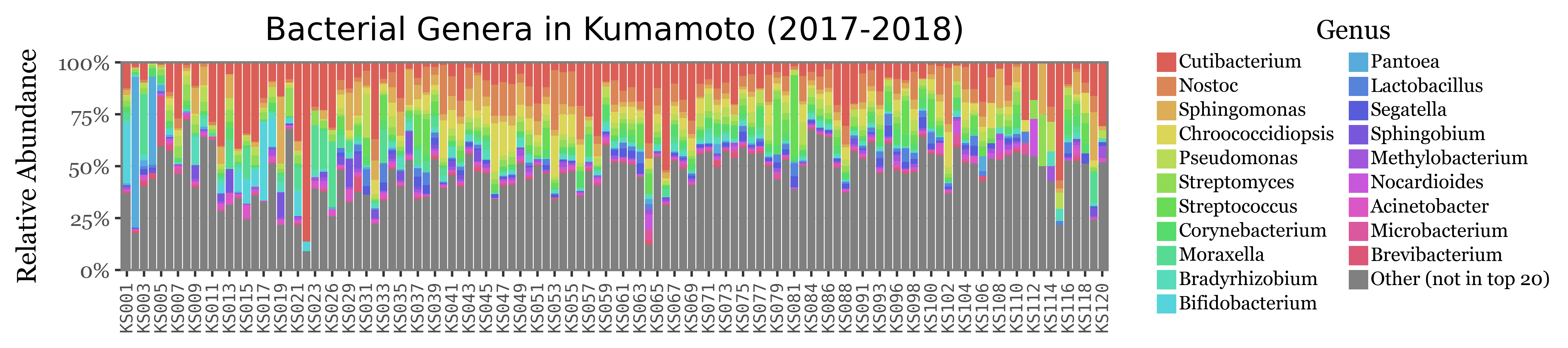
If we now show the most common genera for both Bacteria and Fungi:
Show Code
(kumamoto_genera
 .query('Kingdom=="Bacteria"')
 .query('reads > 0')
 .assign(Genus=lambda dd: np.where(dd.Genus.isin(top_genera['Genus']), dd.Genus,
                                   'Other (not in top 20)'))
 .assign(Genus=lambda dd: pd.Categorical(
    dd.Genus, categories=top_genera.Genus[:20].to_list() + ['Other (not in top 20)'], ordered=True))
 .pipe(lambda dd: p9.ggplot(dd)
 + p9.aes(x='sample_id', y='relative_abundance')
 + p9.geom_col(p9.aes(fill='Genus'))
 + p9.labs(x='', y='Relative Abundance', title='Bacterial Genera in Kumamoto (2017-2018)')
 + p9.scale_fill_manual(discrete_colors)
 + p9.scale_y_continuous(expand=(.0, 0, .0, 0), labels=percent_format())
 + p9.scale_x_discrete(breaks=sorted(dd.sample_id.unique())[::2])
 + p9.theme(figure_size=(9, 2),
            legend_key_size=8,
            legend_text=p9.element_text(size=8),
            legend_title=p9.element_text(ha='center'),
            plot_title=p9.element_text(ha='center', family='Merriweather'),
            axis_text_x=p9.element_text(angle=90, size=7, family='monospace'),
 )
 )
)
Show Code
(kumamoto_genera
 .query('Kingdom=="Fungi"')
 .query('reads > 0')
 .assign(Genus=lambda dd: np.where(dd.Genus.isin(top_genera['Genus']), dd.Genus,
                                   'Other (not in top 20)'))
 .assign(Genus=lambda dd: pd.Categorical(
    dd.Genus, categories=top_genera.Genus[20:].to_list() + ['Other (not in top 20)'], ordered=True))
 .pipe(lambda dd: p9.ggplot(dd)
 + p9.aes(x='sample_id', y='relative_abundance')
 + p9.geom_col(p9.aes(fill='Genus'))
 + p9.labs(x='', y='Relative Abundance', title='Fungal Genera in Kumamoto (2017-2018)')
 + p9.scale_fill_manual(discrete_colors)
 + p9.scale_y_continuous(expand=(.0, 0, .0, 0), labels=percent_format())
 + p9.scale_x_discrete(breaks=sorted(dd.sample_id.unique())[::2])
 + p9.theme(figure_size=(9, 2),
            legend_key_size=8,
            legend_text=p9.element_text(size=8),
            legend_title=p9.element_text(ha='center'),
            plot_title=p9.element_text(ha='center', family='Merriweather'),
            axis_text_x=p9.element_text(angle=90, size=7, family='monospace'),
 )
 ))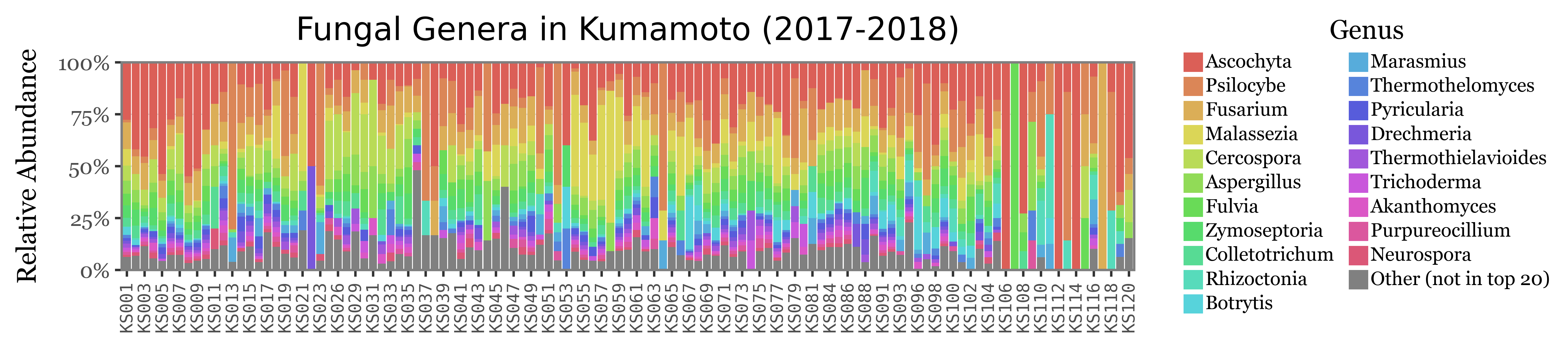
The composition of the relative abundances, while variable, shows much more stability across samples than the total reads assigned to each kingdom. This is a good indication that the relative abundances might be a better proxy for the actual composition of the samples.
Another fact that is evident is that the diversity of bacteria is much higher than the diversity of fungi, which is patent by the % of reads assigned to the “Other” category, which is much higher for bacteria than fungi, which can mostly be explained by its top 20 most common genera.
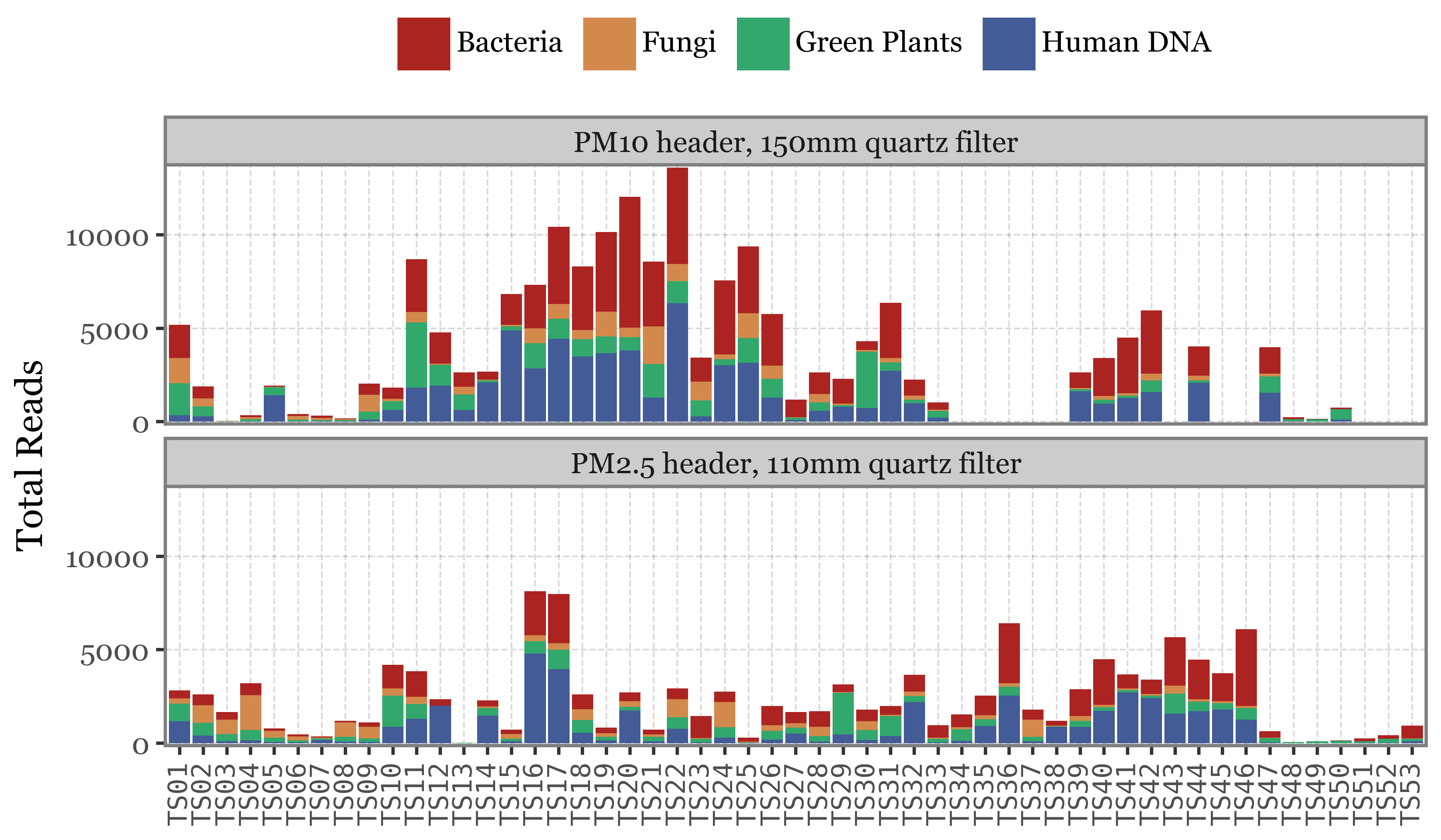
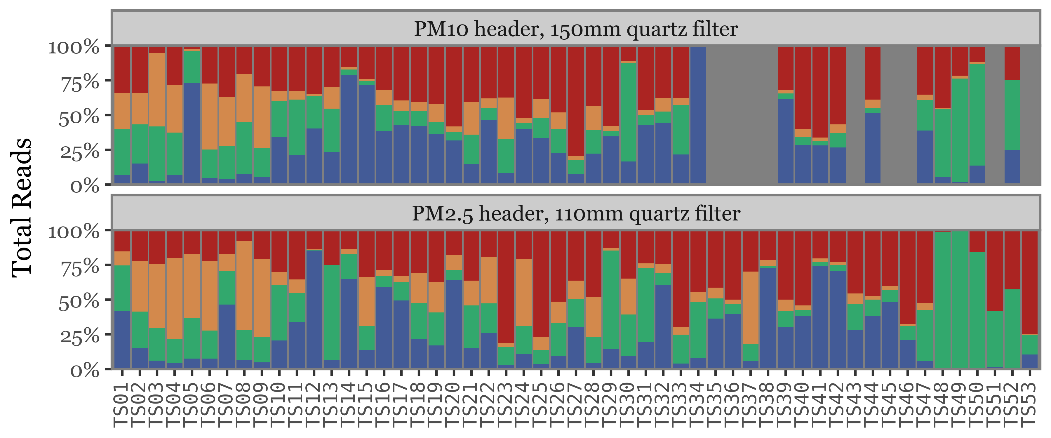
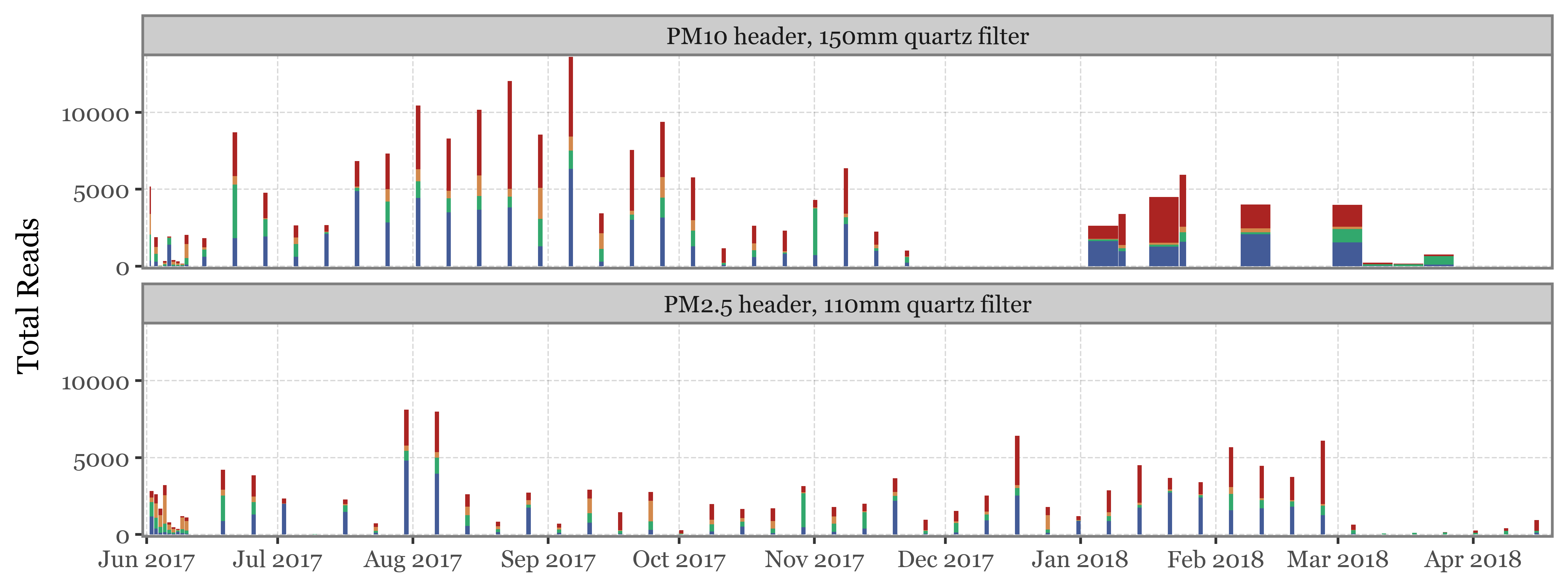
Toyama
We’ll now do the same composition analysis for Toyama, starting with the high taxonomic level:
Show Code
toyama_kingdoms = (pd.concat([
    clean_toyama.query('rank.isin(["Kingdom"])'),
    kingdom_bacteria_toyama.drop(columns=['location', 'sample_type', 'header'])])
 .query('Superkingdom != "Viruses"')
 .query('Superkingdom != "Archaea"')
 .query('rank=="Kingdom"')
 .merge(samples_info, on='sample_id')
 .groupby(['sample_id'])
 .apply(lambda dd: dd.assign(relative_abundance=(dd.reads / dd.reads.sum()).fillna(0)))
 .replace({'Kingdom': {'Metazoa': 'Human DNA', 'Viridiplantae': 'Green Plants'}})
.assign(sample_id=lambda dd: 'TS' + dd.sample_id.str.split('.').str[0].str[2:].str.zfill(2))
 .replace({'PM10': 'PM10 header, 150mm quartz filter',
           'PM2.5': 'PM2.5 header, 110mm quartz filter'})
 .assign(center_date=lambda dd: dd.start_dt + pd.to_timedelta(dd.duration / 2, unit='h'))

)
(toyama_kingdoms
 .pipe(lambda dd: p9.ggplot(dd) + p9.aes(x='sample_id', y='reads')
       + p9.geom_col(p9.aes(fill='Kingdom'))
       + p9.scale_y_continuous(expand=(.01, 0, .01, 0))
       + p9.scale_fill_manual(['#ab2422', '#D3894C', '#32a86d', '#435B97'])
       + p9.facet_wrap('~ header', ncol=1)
    #    + p9.scale_x_discrete(breaks=sorted(dd.sample_id.unique())[::2])
       + p9.labs(x='', y='Total Reads', fill='')
       + p9.theme(
           axis_text_x=p9.element_text(angle=90, size=8, family='monospace'),
           legend_position='top',
           figure_size=(6, 3.5)
       )
       )
)
Show Code
(toyama_kingdoms
 .pipe(lambda dd: p9.ggplot(dd) + p9.aes(x='sample_id', y='relative_abundance')
       + p9.geom_col(p9.aes(fill='Kingdom'))
       + p9.scale_y_continuous(expand=(.0, 0, .0, 0), labels=percent_format())
       + p9.scale_fill_manual(['#ab2422', '#D3894C', '#32a86d', '#435B97'])
       + p9.facet_wrap('~ header', ncol=1)
       + p9.labs(x='', y='Total Reads', fill='')
       + p9.guides(fill=False)
       + p9.theme(
           axis_text_x=p9.element_text(angle=90, size=8, family='monospace'),
           legend_position='top',
           figure_size=(6, 2.5),
           panel_background=p9.element_rect(fill='gray'),
           panel_grid=p9.element_blank()
       )
       )
)
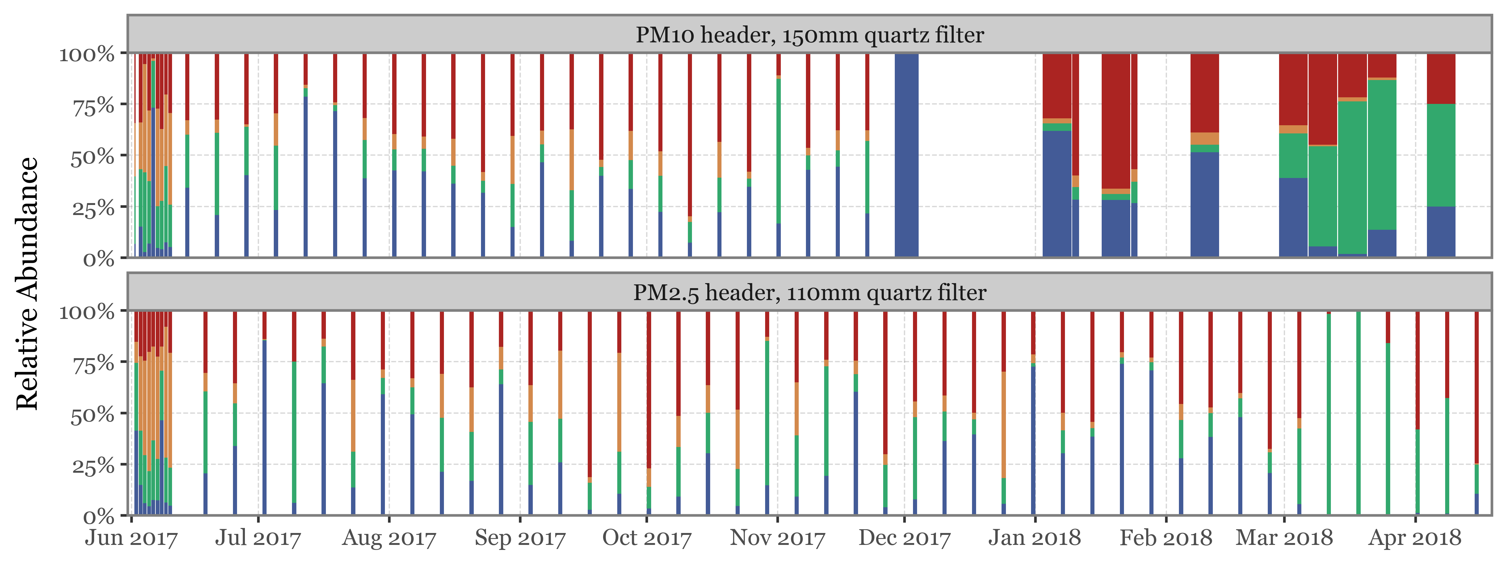
Show Code
(toyama_kingdoms
  .pipe(lambda dd: p9.ggplot(dd) + p9.aes(x='sample_id', y='reads')
       + p9.geom_col(p9.aes(fill='Kingdom', x='center_date', width='duration / 24'))
       + p9.scale_y_continuous(expand=(.01, 0, .01, 0))
       + p9.facet_wrap('~ header', ncol=1)
       + p9.scale_fill_manual(['#ab2422', '#D3894C', '#32a86d', '#435B97'])
       + p9.scale_x_datetime(expand=(.005,  0, .005, 0), date_breaks='1 month', date_labels='%b %Y')
       + p9.labs(x='', y='Total Reads', fill='')
       + p9.guides(fill=False)
       + p9.theme(
           legend_position='top',
           figure_size=(8, 3),
       )
       )
)
Show Code
(toyama_kingdoms
  .pipe(lambda dd: p9.ggplot(dd) + p9.aes(x='sample_id', y='relative_abundance')
       + p9.geom_col(p9.aes(fill='Kingdom', x='center_date', width='duration / 24'))
       + p9.scale_y_continuous(expand=(.0, 0, .0, 0), labels=percent_format())
       + p9.facet_wrap('~ header', ncol=1)
       + p9.scale_fill_manual(['#ab2422', '#D3894C', '#32a86d', '#435B97'])
       + p9.scale_x_datetime(expand=(.005,  0, .005, 0), date_breaks='1 month', date_labels='%b %Y')
       + p9.labs(x='', y='Relative Abundance', fill='')
       + p9.guides(fill=False)
       + p9.theme(
           legend_position='top',
           figure_size=(8, 3),
       )
       )
)
Genus level
Code for data wrangling of Genera
toyama_genera = (clean_toyama
.merge(samples_info)
.query('sample_id.str.startswith("TS")')
.assign(Kingdom=lambda dd: np.where(dd.Superkingdom == 'Bacteria', 'Bacteria', dd.Kingdom))
.query('Superkingdom != "Viruses"')
.query('Superkingdom != "Archaea"')
.query('Kingdom.isin(["Bacteria", "Fungi"])')
.query('rank=="Genus"')
.groupby(['sample_id', 'Kingdom'], as_index=False)
.apply(lambda dd: dd.assign(relative_abundance=dd.reads / dd.reads.sum()))
.drop(columns=['Species'])
.assign(sample_id=lambda dd: 'TS' + dd.sample_id.str.split('.').str[0].str[2:].str.zfill(2))
.replace({'PM10': 'PM10 header, 150mm quartz filter',
'PM2.5': 'PM2.5 header, 110mm quartz filter'})
.assign(center_date=lambda dd: dd.start_dt + pd.to_timedelta(dd.duration / 2, unit='h'))
)
top_genera_toyama = (toyama_genera
.groupby(['Kingdom', 'Genus'])
.agg({'relative_abundance': 'mean', 'reads': 'sum'})
.groupby('Kingdom', group_keys=False)
.apply(lambda dd: dd.nlargest(20, 'relative_abundance'))
.reset_index()
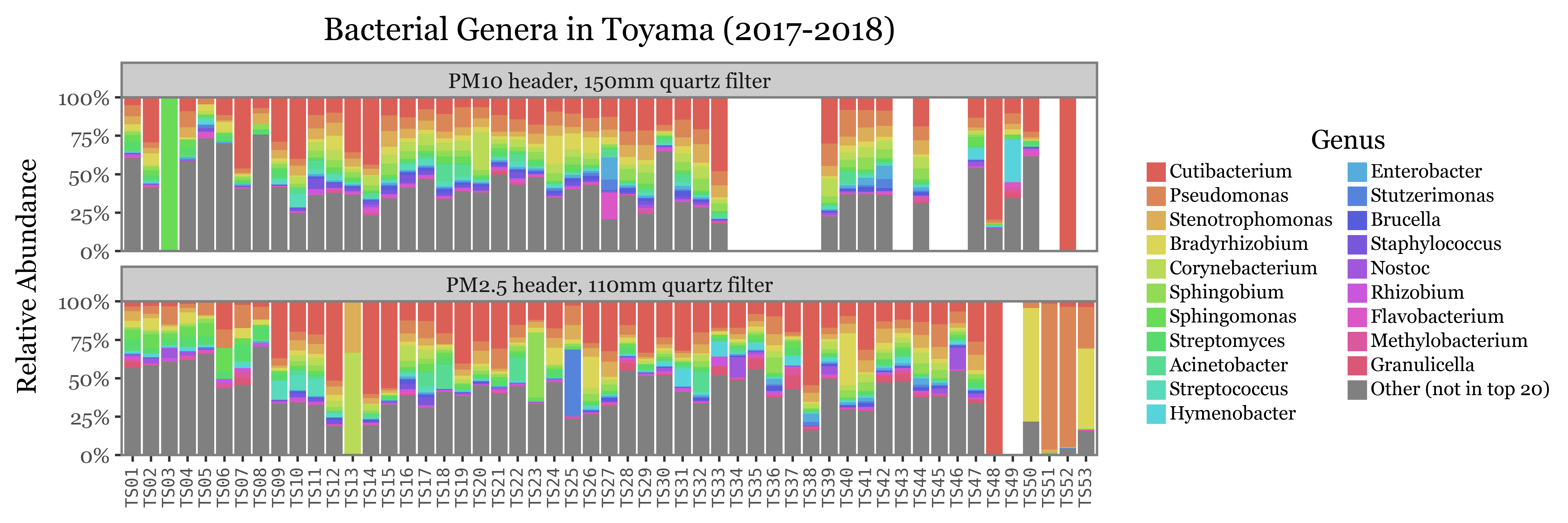
)Show Code
(toyama_genera
 .query('Kingdom=="Bacteria"')
 .query('reads > 0')
 .assign(Genus=lambda dd: np.where(dd.Genus.isin(top_genera_toyama['Genus']), dd.Genus,
                                   'Other (not in top 20)'))
 .assign(Genus=lambda dd: pd.Categorical(
    dd.Genus, categories=top_genera_toyama.Genus[:20].to_list() + ['Other (not in top 20)'], ordered=True))
 .pipe(lambda dd: p9.ggplot(dd)
 + p9.aes(x='sample_id', y='relative_abundance')
 + p9.geom_col(p9.aes(fill='Genus'))
 + p9.labs(x='', y='Relative Abundance', title='Bacterial Genera in Toyama (2017-2018)')
 + p9.scale_fill_manual(discrete_colors)
 + p9.scale_y_continuous(expand=(.0, 0, .0, 0), labels=percent_format())
#  + p9.scale_x_discrete(breaks=sorted(dd.sample_id.unique())[::2])
 + p9.facet_wrap('~ header', ncol=1)
 + p9.theme(figure_size=(9, 3),
            legend_key_size=8,
            legend_text=p9.element_text(size=8),
            legend_title=p9.element_text(ha='center'),
            axis_text_x=p9.element_text(angle=90, size=7, family='monospace'),
            panel_grid=p9.element_blank()
 )
 )
)
kumamoto_all| #perc | tot_all | tot_lvl | 1_all | 1_lvl | 2_all | 2_lvl | 3_all | 3_lvl | 4_all | 4_lvl | 5_all | 5_lvl | 6_all | 6_lvl | 7_all | 7_lvl | 8_all | 8_lvl | 9_all | 9_lvl | 10_all | 10_lvl | 11_all | 11_lvl | 12_all | 12_lvl | 13_all | 13_lvl | 14_all | 14_lvl | 15_all | 15_lvl | 16_all | 16_lvl | 17_all | 17_lvl | 18_all | 18_lvl | 19_all | 19_lvl | 20_all | 20_lvl | 21_all | 21_lvl | 114_all | 114_lvl | 115_all | 115_lvl | 116_all | 116_lvl | 117_all | 117_lvl | 118_all | 118_lvl | 119_all | 119_lvl | 120_all | 120_lvl | 121_all | 121_lvl | 122_all | 122_lvl | 123_all | 123_lvl | 124_all | 124_lvl | 125_all | 125_lvl | 126_all | 126_lvl | 127_all | 127_lvl | 128_all | 128_lvl | 129_all | 129_lvl | 130_all | 130_lvl | 131_all | 131_lvl | 132_all | 132_lvl | 133_all | 133_lvl | 134_all | 134_lvl | lvl_type | taxid | name |
|---|---|---|---|---|---|---|---|---|---|---|---|---|---|---|---|---|---|---|---|---|---|---|---|---|---|---|---|---|---|---|---|---|---|---|---|---|---|---|---|---|---|---|---|---|---|---|---|---|---|---|---|---|---|---|---|---|---|---|---|---|---|---|---|---|---|---|---|---|---|---|---|---|---|---|---|---|---|---|---|---|---|---|---|---|---|---|---|---|---|
|
Loading ITables v2.1.4 from the init_notebook_mode cell...
(need help?) |
pacbio_metrics| sample_id | dna_total | n_reads | total_bases | rl_median | qc_mean | header | sample_type |
|---|---|---|---|---|---|---|---|
|
Loading ITables v2.1.4 from the init_notebook_mode cell...
(need help?) |
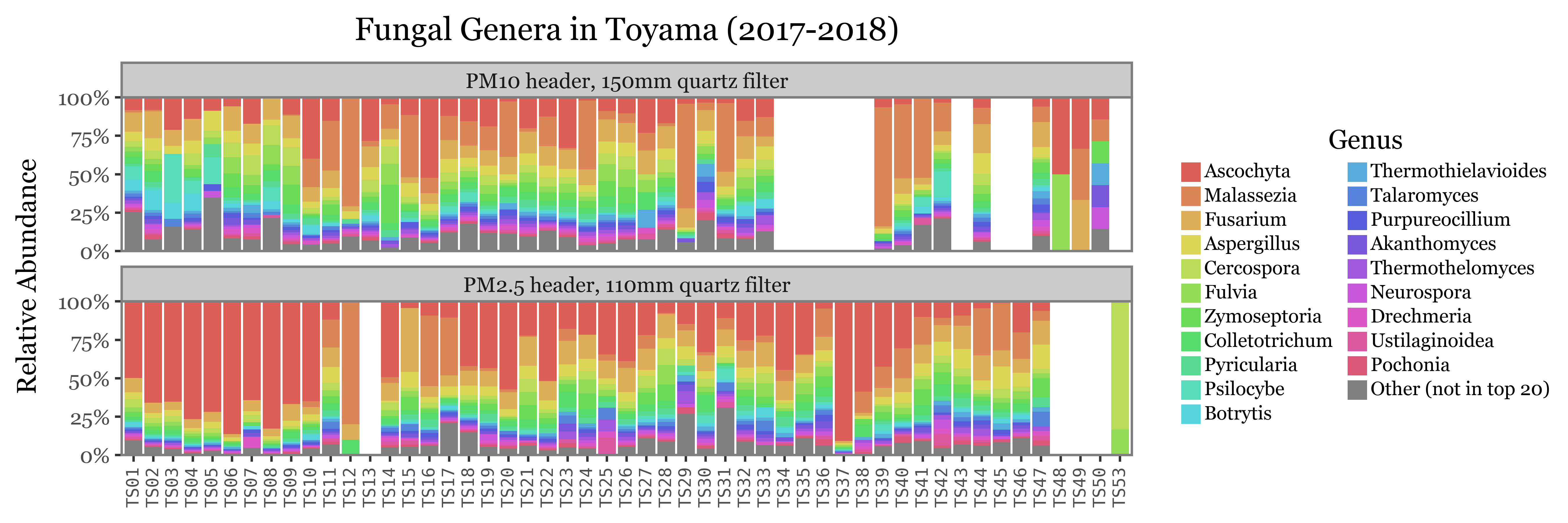
Show Code
(toyama_genera
 .query('Kingdom=="Fungi"')
 .query('reads > 0')
 .assign(Genus=lambda dd: np.where(dd.Genus.isin(top_genera_toyama['Genus']), dd.Genus,
                                   'Other (not in top 20)'))
 .assign(Genus=lambda dd: pd.Categorical(
    dd.Genus, categories=top_genera_toyama.Genus[20:].to_list() + ['Other (not in top 20)'], ordered=True))
 .pipe(lambda dd: p9.ggplot(dd)
 + p9.aes(x='sample_id', y='relative_abundance')
 + p9.geom_col(p9.aes(fill='Genus'))
 + p9.labs(x='', y='Relative Abundance', title='Fungal Genera in Toyama (2017-2018)')
 + p9.scale_fill_manual(discrete_colors)
 + p9.scale_y_continuous(expand=(.0, 0, .0, 0), labels=percent_format())
#  + p9.scale_x_discrete(breaks=sorted(dd.sample_id.unique())[::2])
 + p9.facet_wrap('~ header', ncol=1)
 + p9.theme(figure_size=(9, 3),
            legend_key_size=8,
            legend_text=p9.element_text(size=8),
            legend_title=p9.element_text(ha='center'),
            axis_text_x=p9.element_text(angle=90, size=7, family='monospace'),
            panel_grid=p9.element_blank()
 )
 )
)
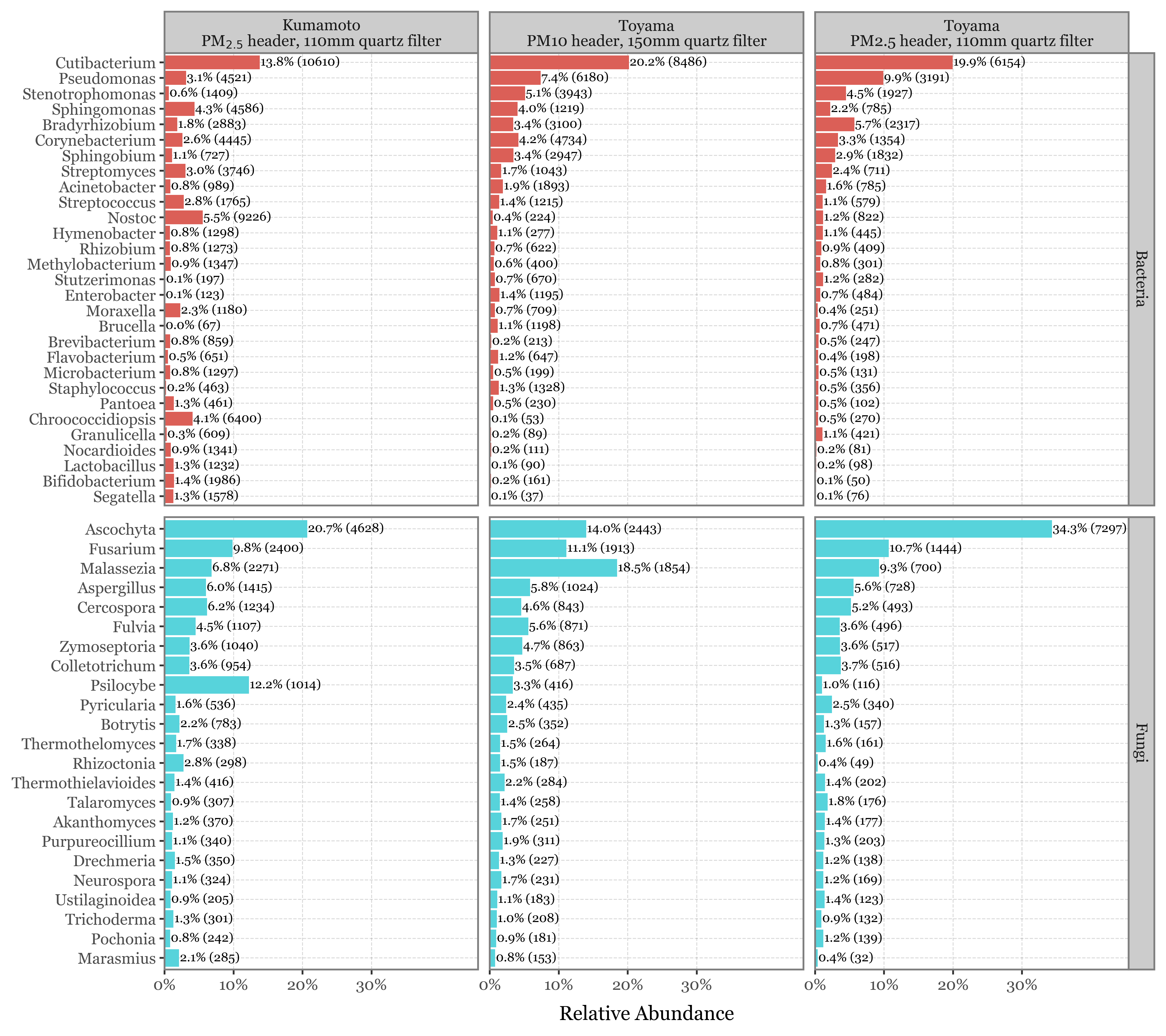
Comparison between Toyama, Kumamoto and header types
I have computed the 20 most common genera for both Bacteria and Fungi in Toyama and Kumamoto separately. That makes a total of 29 bacterial genera and 23 fungal genera which are very common in the samples of either site.
If we now compare the average relative abundance of these genera in both sites and header type (showing the total reads assigned to each Genus for context since the total reads variability is huge):
Show Code
all_top_genera = set(top_genera['Genus'].to_list() + top_genera_toyama['Genus'].to_list())
top_genera_union_toyama = (toyama_genera
 .query('rank=="Genus"')
 .assign(Genus=lambda dd: np.where(dd.Genus.isin(all_top_genera), dd.Genus,
                                   'Other'))
 .groupby(['Kingdom', 'Genus', 'header'])
 .agg({'relative_abundance': 'mean', 'reads': 'sum'})
  .query('Genus != "Other"')
)

top_genera_union_kumamoto = (kumamoto_genera
                     .query('rank=="Genus"')
                     .assign(Genus=lambda dd: np.where(dd.Genus.isin(all_top_genera), dd.Genus,
                                   'Other'))
                     .assign(header='PM$_{2.5}$ header, 110mm quartz filter')
                     .groupby(['Kingdom', 'Genus', 'header'])
 .agg({'relative_abundance': 'mean', 'reads': 'sum'})
 .query('Genus != "Other"')
)

(pd.concat([
    top_genera_union_kumamoto.assign(location='Kumamoto'),
    top_genera_union_toyama.assign(location='Toyama')
])
.reset_index()
.assign(percent_label=lambda dd: (dd['relative_abundance'] * 100).round(1).astype(str)
        + '%' + ' (' + dd['reads'].astype(str) + ')')
.pipe(lambda dd: p9.ggplot(dd)
        + p9.aes('reorder(Genus, relative_abundance)', 'relative_abundance')
        + p9.geom_col(p9.aes(fill='Kingdom'))
        + p9.geom_text(p9.aes(label='percent_label'), size=7, nudge_y=.001, ha='left')
        + p9.coord_flip()
        + p9.scale_y_continuous(labels=percent_format(), expand=(0, 0, .32, 0),
                                breaks=[0, .1, .2, .3])
        + p9.guides(fill=False)
        + p9.labs(x='', y='Relative Abundance')
        + p9.facet_grid('Kingdom ~ location + header', scales='free_y')
        + p9.theme(figure_size=(9, 8)
                   )
      )
)
Computation of statistics for the top genera
kumamoto_genera_stats = (kumamoto_genera
                     .query('rank=="Genus"')
                     .assign(header='PM$_{2.5}$ header, 110mm quartz filter')
                     .groupby(['Kingdom', 'Genus', 'header'], as_index=False)
 .agg({'relative_abundance': 'mean'})
 .drop(columns='header')
)

toyama_genera_pm25_stats = (toyama_genera
                     .query('rank=="Genus"')
                     .groupby(['Kingdom', 'Genus', 'header'], as_index=False)
 .agg({'relative_abundance': 'mean'})
 .query('header=="PM2.5 header, 110mm quartz filter"')
    .drop(columns='header')
)

toyama_genera_pm10_stats = (toyama_genera
                        .query('rank=="Genus"')
                        .groupby(['Kingdom', 'Genus', 'header'], as_index=False)
    .agg({'relative_abundance': 'mean'})
    .query('header=="PM10 header, 150mm quartz filter"')
        .drop(columns='header')
    )
Kumamoto vs Toyama
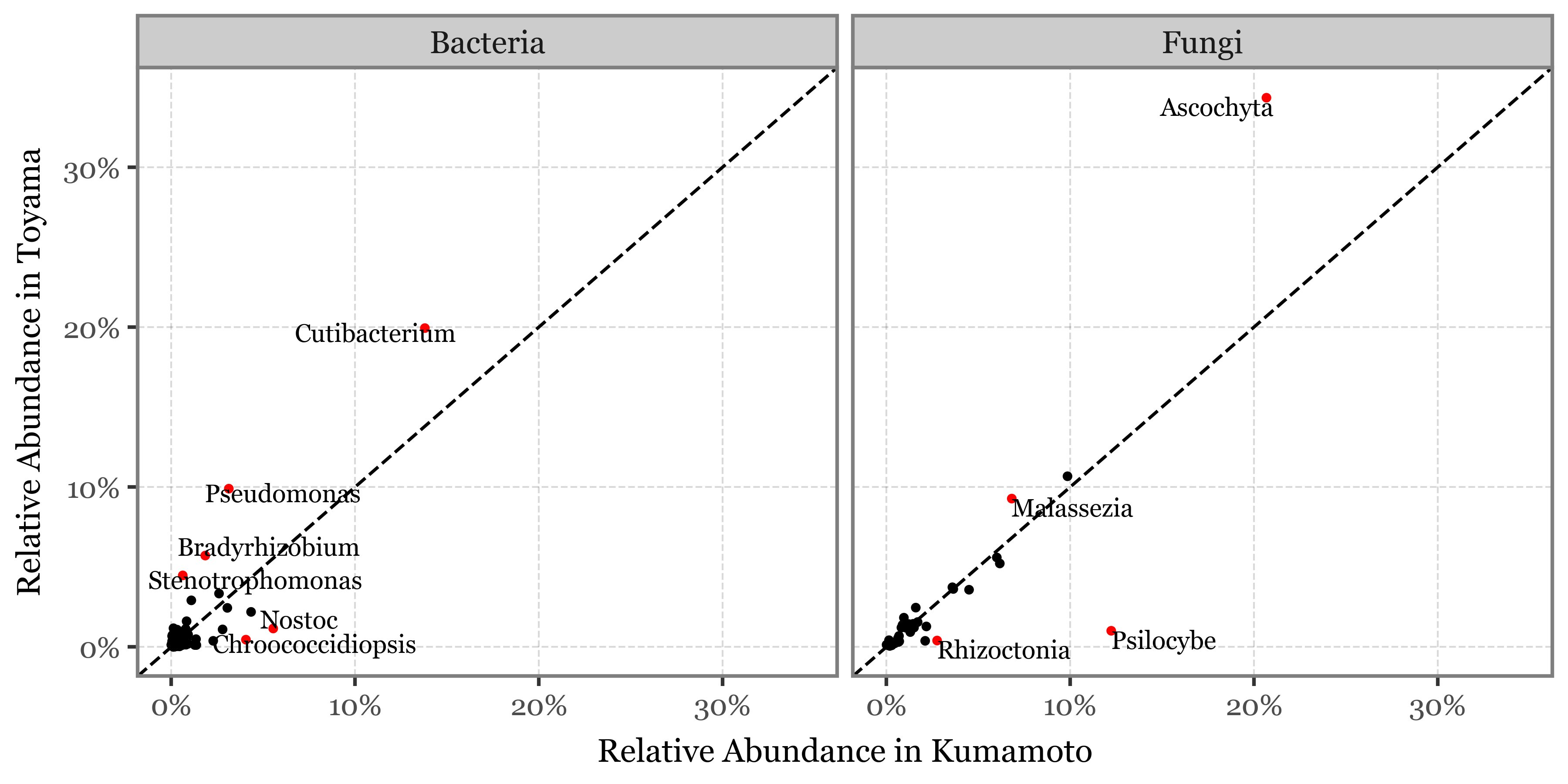
I’ve just showcased the genera with the highest difference in each case between the samples taken with the 2.5 um header in Toyama and Kumamoto:
Show Code
kumamoto_toyama_comp = (kumamoto_genera_stats
 .merge(toyama_genera_pm25_stats, on=['Kingdom', 'Genus'], suffixes=('_kumamoto', '_toyama'))
 .loc[lambda dd: (dd.relative_abundance_kumamoto > .001) | (dd.relative_abundance_toyama > .001)]
 .eval('ratio = relative_abundance_toyama / relative_abundance_kumamoto')
 .assign(log_ratio=lambda dd: np.log2(dd['ratio']))
 .eval('diff = relative_abundance_toyama - relative_abundance_kumamoto')
 .eval('selected = log_ratio.abs() > 3 or diff.abs() > .02')
 .eval('combined = log_ratio.abs() * diff.abs()')
 .eval('abs_diff = diff.abs()')
)

top_selected = kumamoto_toyama_comp.sort_values('abs_diff', ascending=False).head(10).query('selected')


(kumamoto_toyama_comp
.pipe(lambda dd: p9.ggplot(dd)
    + p9.aes('relative_abundance_kumamoto', 'relative_abundance_toyama')
    + p9.geom_point(p9.aes(color='Genus.isin(top_selected.Genus)'), stroke=0, size=1.5)
    + p9.scale_x_continuous(labels=percent_format(), limits=(-.001, .345))
    + p9.scale_y_continuous(labels=percent_format(), limits=(-.001, .345))
    + p9.geom_text(p9.aes(label='Genus'), size=7, data=top_selected, ha='left',
                    adjust_text={'expand': (1.5, 1.5), 'arrowprops': dict(arrowstyle='-', lw=0)})
    + p9.scale_color_manual({True: 'red', False: 'black'})
    + p9.guides(color=False)
    + p9.facet_wrap('Kingdom')
    + p9.geom_abline(intercept=0, slope=1, linetype='dashed')
    + p9.labs(x='Relative Abundance in Kumamoto', y='Relative Abundance in Toyama',
                color='Relative Abundance Difference', size='Log2(Ratio)')
    + p9.theme(figure_size=(6, 3),
               axis_text=p9.element_text(size=8),
               axis_title=p9.element_text(size=9),
    )
    )
)
The full table with different metrics of difference is the following:
Show Code
show(kumamoto_toyama_comp
 .rename(columns={'relative_abundance_kumamoto': 'RA Kumamoto', 'relative_abundance_toyama': 'RA Toyama'})
 .sort_values('combined', ascending=False)
 [['Kingdom', 'Genus', 'RA Kumamoto', 'RA Toyama', 'abs_diff', 'ratio', 'log_ratio']]
 .style.format({'log_ratio': '{:.2f}', 'abs_diff': lambda x: f"{x * 100:.2f}", 'ratio': '{:.2f}',
                'RA Kumamoto': '{:.2%}', 'RA Toyama': '{:.2%}'})
 .hide(axis=0),
 buttons=['csv', 'colvis'], pageLength=20
)| Kingdom | Genus | RA Kumamoto | RA Toyama | abs_diff | ratio | log_ratio |
|---|---|---|---|---|---|---|
| Fungi | Psilocybe | 12.23% | 2.10% | 10.13 | 0.17 | -2.54 |
| Bacteria | Chroococcidiopsis | 4.06% | 0.29% | 3.76 | 0.07 | -3.78 |
| Bacteria | Nostoc | 5.54% | 0.83% | 4.72 | 0.15 | -2.75 |
| Bacteria | Stenotrophomonas | 0.62% | 4.77% | 4.15 | 7.69 | 2.94 |
| Bacteria | Pseudomonas | 3.13% | 8.75% | 5.63 | 2.80 | 1.49 |
| Fungi | Malassezia | 6.82% | 13.61% | 6.79 | 2.00 | 1.00 |
| Bacteria | Segatella | 1.27% | 0.09% | 1.19 | 0.07 | -3.87 |
| Bacteria | Bifidobacterium | 1.36% | 0.14% | 1.22 | 0.10 | -3.32 |
| Bacteria | Enterobacter | 0.06% | 1.04% | 0.98 | 16.94 | 4.08 |
| Bacteria | Lactobacillus | 1.30% | 0.13% | 1.17 | 0.10 | -3.30 |
| Bacteria | Brucella | 0.04% | 0.89% | 0.85 | 21.99 | 4.46 |
| Bacteria | Bradyrhizobium | 1.85% | 4.66% | 2.81 | 2.52 | 1.34 |
| Bacteria | Moraxella | 2.28% | 0.54% | 1.74 | 0.24 | -2.08 |
| Bacteria | Cutibacterium | 13.80% | 20.04% | 6.24 | 1.45 | 0.54 |
| Bacteria | Sphingobium | 1.09% | 3.14% | 2.06 | 2.89 | 1.53 |
| Fungi | Rhizoctonia | 2.75% | 0.91% | 1.84 | 0.33 | -1.59 |
| Fungi | Marasmius | 2.11% | 0.57% | 1.54 | 0.27 | -1.89 |
| Bacteria | Stutzerimonas | 0.12% | 0.98% | 0.86 | 8.43 | 3.07 |
| Bacteria | Streptococcus | 2.79% | 1.21% | 1.58 | 0.43 | -1.20 |
| Bacteria | Ensifer | 0.04% | 0.54% | 0.50 | 12.71 | 3.67 |
| Bacteria | Limosilactobacillus | 0.44% | 0.02% | 0.42 | 0.05 | -4.33 |
| Bacteria | Nocardioides | 0.90% | 0.20% | 0.70 | 0.22 | -2.19 |
| Bacteria | Brasilonema | 0.49% | 0.05% | 0.44 | 0.10 | -3.36 |
| Bacteria | Clostridium | 0.80% | 0.17% | 0.63 | 0.21 | -2.24 |
| Bacteria | Pantoea | 1.34% | 0.48% | 0.86 | 0.36 | -1.48 |
| Bacteria | Staphylococcus | 0.23% | 0.86% | 0.62 | 3.70 | 1.89 |
| Bacteria | Caulobacter | 0.07% | 0.47% | 0.40 | 6.97 | 2.80 |
| Bacteria | Tessaracoccus | 0.35% | 0.03% | 0.32 | 0.10 | -3.39 |
| Fungi | Ascochyta | 20.68% | 24.72% | 4.05 | 1.20 | 0.26 |
| Bacteria | Faecalibacterium | 0.42% | 0.06% | 0.36 | 0.14 | -2.79 |
| Bacteria | Acinetobacter | 0.83% | 1.74% | 0.91 | 2.10 | 1.07 |
| Bacteria | Enhydrobacter | 0.02% | 0.28% | 0.26 | 13.26 | 3.73 |
| Bacteria | Bacteroides | 0.61% | 0.15% | 0.46 | 0.25 | -2.02 |
| Bacteria | Janibacter | 0.37% | 0.05% | 0.32 | 0.14 | -2.87 |
| Bacteria | Gibbsiella | 0.15% | 0.00% | 0.15 | 0.02 | -5.49 |
| Bacteria | Megasphaera | 0.22% | 0.01% | 0.20 | 0.07 | -3.89 |
| Bacteria | Sneathiella | 0.00% | 0.13% | 0.13 | 60.09 | 5.91 |
| Bacteria | Lawsonella | 0.02% | 0.23% | 0.21 | 11.78 | 3.56 |
| Fungi | Debaryomyces | 0.14% | 0.51% | 0.38 | 3.77 | 1.92 |
| Bacteria | Brevundimonas | 0.17% | 0.57% | 0.40 | 3.39 | 1.76 |
| Bacteria | Shewanella | 0.13% | 0.50% | 0.37 | 3.76 | 1.91 |
| Bacteria | Sphingomonas | 4.34% | 3.02% | 1.32 | 0.70 | -0.52 |
| Bacteria | Thiosulfatimonas | 0.11% | 0.00% | 0.11 | 0.01 | -6.17 |
| Bacteria | Prevotella | 0.68% | 0.24% | 0.44 | 0.36 | -1.48 |
| Bacteria | Latilactobacillus | 0.01% | 0.14% | 0.13 | 24.94 | 4.64 |
| Bacteria | Corynebacterium | 2.59% | 3.71% | 1.11 | 1.43 | 0.51 |
| Bacteria | Deinococcus | 0.52% | 0.17% | 0.35 | 0.33 | -1.61 |
| Bacteria | Denitrificimonas | 0.12% | 0.00% | 0.11 | 0.03 | -5.02 |
| Fungi | Talaromyces | 0.95% | 1.65% | 0.70 | 1.74 | 0.80 |
| Bacteria | Blautia | 0.27% | 0.05% | 0.22 | 0.18 | -2.47 |
| Bacteria | Oscillatoria | 0.18% | 0.02% | 0.16 | 0.10 | -3.30 |
| Bacteria | Streptomyces | 3.05% | 2.09% | 0.96 | 0.69 | -0.55 |
| Bacteria | Glutamicibacter | 0.25% | 0.04% | 0.20 | 0.18 | -2.49 |
| Fungi | Pyricularia | 1.59% | 2.42% | 0.83 | 1.52 | 0.60 |
| Bacteria | Brevibacterium | 0.80% | 0.37% | 0.43 | 0.47 | -1.10 |
| Bacteria | Leuconostoc | 0.07% | 0.29% | 0.22 | 4.14 | 2.05 |
| Bacteria | Cylindrospermum | 0.16% | 0.02% | 0.14 | 0.12 | -3.08 |
| Bacteria | Calothrix | 0.25% | 0.05% | 0.19 | 0.21 | -2.23 |
| Bacteria | Gordonia | 0.25% | 0.59% | 0.34 | 2.37 | 1.24 |
| Bacteria | Mediterraneibacter | 0.16% | 0.02% | 0.14 | 0.12 | -3.07 |
| Fungi | Cercospora | 6.17% | 4.91% | 1.25 | 0.80 | -0.33 |
| Bacteria | Gloeocapsa | 0.15% | 0.02% | 0.14 | 0.13 | -2.99 |
| Bacteria | Dyella | 0.14% | 0.02% | 0.13 | 0.11 | -3.16 |
| Bacteria | Vescimonas | 0.12% | 0.01% | 0.11 | 0.08 | -3.69 |
| Bacteria | Granulicella | 0.31% | 0.67% | 0.36 | 2.14 | 1.10 |
| Bacteria | Leucobacter | 0.17% | 0.03% | 0.14 | 0.16 | -2.66 |
| Bacteria | Lacipirellula | 0.05% | 0.22% | 0.17 | 4.51 | 2.17 |
| Bacteria | Alistipes | 0.20% | 0.04% | 0.16 | 0.20 | -2.33 |
| Bacteria | Hyphomicrobium | 0.25% | 0.07% | 0.19 | 0.27 | -1.91 |
| Bacteria | Flavonifractor | 0.12% | 0.01% | 0.10 | 0.10 | -3.26 |
| Bacteria | Edaphobacter | 0.08% | 0.27% | 0.19 | 3.24 | 1.69 |
| Bacteria | Lachnoclostridium | 0.12% | 0.01% | 0.10 | 0.13 | -2.98 |
| Bacteria | Halotia | 0.13% | 0.02% | 0.11 | 0.16 | -2.65 |
| Fungi | Saccharomyces | 0.44% | 0.19% | 0.25 | 0.44 | -1.19 |
| Bacteria | Brachybacterium | 0.25% | 0.08% | 0.17 | 0.31 | -1.68 |
| Bacteria | Terriglobus | 0.30% | 0.59% | 0.29 | 1.97 | 0.98 |
| Bacteria | Leptolyngbya | 0.25% | 0.08% | 0.17 | 0.32 | -1.65 |
| Bacteria | Allocoleopsis | 0.17% | 0.04% | 0.13 | 0.24 | -2.04 |
| Bacteria | Rubrobacter | 0.19% | 0.05% | 0.14 | 0.26 | -1.93 |
| Fungi | Purpureocillium | 1.10% | 1.59% | 0.49 | 1.45 | 0.54 |
| Bacteria | Collinsella | 0.11% | 0.02% | 0.09 | 0.14 | -2.79 |
| Bacteria | Fibrella | 0.06% | 0.20% | 0.14 | 3.53 | 1.82 |
| Bacteria | Ornithinimicrobium | 0.14% | 0.03% | 0.11 | 0.21 | -2.25 |
| Bacteria | Psychrobacter | 0.23% | 0.07% | 0.15 | 0.32 | -1.64 |
| Bacteria | Ruminococcus | 0.12% | 0.02% | 0.10 | 0.18 | -2.50 |
| Bacteria | Sorangium | 0.25% | 0.09% | 0.16 | 0.35 | -1.52 |
| Bacteria | Microbacterium | 0.82% | 0.50% | 0.32 | 0.61 | -0.72 |
| Bacteria | Tolypothrix | 0.15% | 0.04% | 0.11 | 0.28 | -1.85 |
| Bacteria | Flavisolibacter | 0.15% | 0.04% | 0.11 | 0.28 | -1.82 |
| Bacteria | Flavobacterium | 0.50% | 0.79% | 0.29 | 1.58 | 0.66 |
| Bacteria | Fischerella | 0.13% | 0.04% | 0.10 | 0.26 | -1.92 |
| Fungi | Ustilaginoidea | 0.87% | 1.24% | 0.36 | 1.42 | 0.50 |
| Bacteria | Halopseudomonas | 0.19% | 0.07% | 0.12 | 0.36 | -1.48 |
| Bacteria | Actinomyces | 0.08% | 0.21% | 0.13 | 2.60 | 1.38 |
| Fungi | Kluyveromyces | 0.06% | 0.17% | 0.11 | 2.78 | 1.47 |
| Bacteria | Hymenobacter | 0.78% | 1.10% | 0.32 | 1.41 | 0.50 |
| Bacteria | Porphyromonas | 0.03% | 0.11% | 0.08 | 3.80 | 1.93 |
| Fungi | Yarrowia | 0.28% | 0.14% | 0.15 | 0.49 | -1.04 |
| Bacteria | Ralstonia | 0.09% | 0.22% | 0.12 | 2.33 | 1.22 |
| Bacteria | Neisseria | 0.08% | 0.19% | 0.11 | 2.48 | 1.31 |
| Fungi | Fusarium | 9.85% | 10.88% | 1.03 | 1.10 | 0.14 |
| Bacteria | Burkholderia | 0.56% | 0.34% | 0.21 | 0.62 | -0.69 |
| Bacteria | Mycobacteroides | 0.05% | 0.15% | 0.10 | 2.82 | 1.50 |
| Bacteria | Selenomonas | 0.11% | 0.03% | 0.08 | 0.29 | -1.80 |
| Bacteria | Dietzia | 0.11% | 0.03% | 0.08 | 0.28 | -1.83 |
| Fungi | Neurospora | 1.08% | 1.42% | 0.34 | 1.32 | 0.40 |
| Fungi | Naumovozyma | 0.18% | 0.07% | 0.11 | 0.41 | -1.29 |
| Bacteria | Bordetella | 0.07% | 0.18% | 0.10 | 2.43 | 1.28 |
| Fungi | Sporisorium | 0.65% | 0.43% | 0.22 | 0.66 | -0.60 |
| Fungi | Trichoderma | 1.29% | 0.97% | 0.32 | 0.75 | -0.41 |
| Fungi | Akanthomyces | 1.21% | 1.55% | 0.34 | 1.28 | 0.36 |
| Bacteria | Aeromicrobium | 0.11% | 0.04% | 0.07 | 0.35 | -1.51 |
| Fungi | Pochonia | 0.81% | 1.07% | 0.26 | 1.32 | 0.40 |
| Fungi | Thermothielavioides | 1.45% | 1.78% | 0.33 | 1.23 | 0.30 |
| Bacteria | Chryseobacterium | 0.12% | 0.23% | 0.11 | 1.87 | 0.90 |
| Fungi | Zymoseptoria | 3.64% | 4.14% | 0.51 | 1.14 | 0.19 |
| Bacteria | Phocaeicola | 0.11% | 0.05% | 0.07 | 0.39 | -1.35 |
| Bacteria | Comamonas | 0.22% | 0.12% | 0.10 | 0.54 | -0.89 |
| Bacteria | Methylobacterium | 0.91% | 0.69% | 0.22 | 0.75 | -0.41 |
| Fungi | Candida | 0.12% | 0.21% | 0.10 | 1.84 | 0.88 |
| Fungi | Ustilago | 0.41% | 0.27% | 0.14 | 0.66 | -0.61 |
| Bacteria | Enterococcus | 0.13% | 0.06% | 0.07 | 0.46 | -1.13 |
| Bacteria | Shinella | 0.08% | 0.15% | 0.07 | 1.93 | 0.95 |
| Bacteria | Roseateles | 0.05% | 0.11% | 0.06 | 2.13 | 1.09 |
| Fungi | Botrytis | 2.17% | 1.87% | 0.30 | 0.86 | -0.21 |
| Bacteria | Pseudoalteromonas | 0.06% | 0.11% | 0.06 | 2.08 | 1.05 |
| Fungi | Drechmeria | 1.50% | 1.26% | 0.24 | 0.84 | -0.25 |
| Bacteria | Arthrobacter | 0.36% | 0.25% | 0.11 | 0.70 | -0.52 |
| Fungi | Scheffersomyces | 0.08% | 0.14% | 0.06 | 1.82 | 0.86 |
| Bacteria | Pseudonocardia | 0.10% | 0.05% | 0.05 | 0.49 | -1.04 |
| Bacteria | Bosea | 0.08% | 0.14% | 0.06 | 1.78 | 0.84 |
| Fungi | Brettanomyces | 0.18% | 0.11% | 0.07 | 0.61 | -0.71 |
| Bacteria | Microvirga | 0.13% | 0.07% | 0.06 | 0.55 | -0.87 |
| Fungi | Puccinia | 0.63% | 0.49% | 0.14 | 0.78 | -0.35 |
| Bacteria | Pseudoxanthomonas | 0.35% | 0.47% | 0.12 | 1.33 | 0.41 |
| Bacteria | Sphingopyxis | 0.30% | 0.21% | 0.09 | 0.70 | -0.52 |
| Bacteria | Klebsiella | 0.07% | 0.13% | 0.05 | 1.71 | 0.78 |
| Bacteria | Nocardiopsis | 0.11% | 0.06% | 0.05 | 0.56 | -0.84 |
| Bacteria | Azospirillum | 0.07% | 0.13% | 0.05 | 1.69 | 0.76 |
| Bacteria | Paenibacillus | 0.46% | 0.35% | 0.10 | 0.77 | -0.37 |
| Fungi | Schizosaccharomyces | 0.14% | 0.09% | 0.05 | 0.62 | -0.68 |
| Fungi | Tetrapisispora | 0.08% | 0.14% | 0.05 | 1.61 | 0.69 |
| Bacteria | Massilia | 0.29% | 0.21% | 0.08 | 0.73 | -0.46 |
| Bacteria | Agrobacterium | 0.26% | 0.34% | 0.09 | 1.33 | 0.42 |
| Bacteria | Rothia | 0.09% | 0.13% | 0.05 | 1.56 | 0.64 |
| Bacteria | Citrobacter | 0.06% | 0.10% | 0.04 | 1.63 | 0.71 |
| Bacteria | Actinoplanes | 0.12% | 0.08% | 0.04 | 0.65 | -0.62 |
| Bacteria | Spirosoma | 0.51% | 0.42% | 0.09 | 0.82 | -0.29 |
| Fungi | Thermothelomyces | 1.69% | 1.52% | 0.17 | 0.90 | -0.15 |
| Bacteria | Nocardia | 0.16% | 0.11% | 0.05 | 0.69 | -0.54 |
| Bacteria | Luteibacter | 0.10% | 0.07% | 0.04 | 0.62 | -0.68 |
| Bacteria | Xanthomonas | 0.38% | 0.46% | 0.09 | 1.23 | 0.30 |
| Bacteria | Mycobacterium | 0.36% | 0.28% | 0.07 | 0.80 | -0.33 |
| Bacteria | Amycolatopsis | 0.18% | 0.23% | 0.05 | 1.31 | 0.39 |
| Fungi | Cutaneotrichosporon | 0.69% | 0.60% | 0.10 | 0.86 | -0.22 |
| Fungi | Aspergillus | 6.00% | 5.71% | 0.29 | 0.95 | -0.07 |
| Bacteria | Achromobacter | 0.14% | 0.10% | 0.04 | 0.73 | -0.46 |
| Bacteria | Novosphingobium | 0.37% | 0.30% | 0.06 | 0.83 | -0.27 |
| Fungi | Cryptococcus | 0.66% | 0.75% | 0.09 | 1.14 | 0.19 |
| Bacteria | Microlunatus | 0.14% | 0.10% | 0.04 | 0.74 | -0.44 |
| Bacteria | Devosia | 0.21% | 0.17% | 0.05 | 0.79 | -0.35 |
| Fungi | Penicillium | 0.68% | 0.77% | 0.09 | 1.13 | 0.17 |
| Bacteria | Rhodococcus | 0.39% | 0.45% | 0.07 | 1.17 | 0.23 |
| Fungi | Eremothecium | 0.12% | 0.16% | 0.04 | 1.31 | 0.39 |
| Bacteria | Lysobacter | 0.17% | 0.13% | 0.04 | 0.79 | -0.34 |
| Bacteria | Halomonas | 0.15% | 0.12% | 0.03 | 0.79 | -0.33 |
| Bacteria | Mucilaginibacter | 0.13% | 0.16% | 0.03 | 1.23 | 0.30 |
| Bacteria | Escherichia | 0.09% | 0.12% | 0.03 | 1.27 | 0.34 |
| Bacteria | Paraburkholderia | 0.25% | 0.21% | 0.04 | 0.85 | -0.23 |
| Bacteria | Aeromonas | 0.21% | 0.17% | 0.03 | 0.84 | -0.24 |
| Bacteria | Micromonospora | 0.24% | 0.21% | 0.03 | 0.87 | -0.20 |
| Bacteria | Rhodopseudomonas | 0.11% | 0.09% | 0.02 | 0.83 | -0.27 |
| Bacteria | Kocuria | 0.16% | 0.18% | 0.02 | 1.15 | 0.20 |
| Bacteria | Sinorhizobium | 0.11% | 0.12% | 0.02 | 1.14 | 0.19 |
| Bacteria | Cupriavidus | 0.23% | 0.25% | 0.02 | 1.08 | 0.10 |
| Bacteria | Vibrio | 0.39% | 0.37% | 0.02 | 0.95 | -0.08 |
| Bacteria | Mycolicibacterium | 0.55% | 0.53% | 0.02 | 0.96 | -0.06 |
| Bacteria | Pedobacter | 0.10% | 0.09% | 0.01 | 0.92 | -0.11 |
| Bacteria | Rhizobium | 0.79% | 0.81% | 0.02 | 1.03 | 0.04 |
| Fungi | Colletotrichum | 3.59% | 3.63% | 0.04 | 1.01 | 0.02 |
| Bacteria | Cellulomonas | 0.11% | 0.10% | 0.01 | 0.95 | -0.08 |
| Bacteria | Paracoccus | 0.30% | 0.29% | 0.01 | 0.97 | -0.04 |
| Fungi | Fulvia | 4.49% | 4.52% | 0.03 | 1.01 | 0.01 |
| Bacteria | Variovorax | 0.35% | 0.34% | 0.01 | 0.99 | -0.02 |
| Bacteria | Mesorhizobium | 0.51% | 0.51% | 0.00 | 1.01 | 0.01 |
| Bacteria | Curtobacterium | 0.17% | 0.17% | 0.00 | 1.00 | -0.01 |
| Bacteria | Bacillus | 0.32% | 0.32% | 0.00 | 1.00 | -0.00 |
A more proper way of performing this comparison would be to use ANCOM (analysis of composition of microbiomes). But for the moment, we are just showcasing the differences between the relative abundances for these genera between the two sites. In this case, the top 10 genera with the highest difference in relative abundance between Toyama and Kumamoto (for the samples taken with the 2.5 um header) are the following for both Fungi and Bacteria:
Show Code
(kumamoto_toyama_comp
 .assign(direction=lambda dd: np.where(dd['ratio'] > 1, 'Toyama', 'Kumamoto'))
 .groupby(['direction', 'Kingdom'],  as_index=False)
 .apply(lambda dd: dd.sort_values('abs_diff', ascending=False).head(10))
 [['Kingdom', 'Genus', 'direction', 'relative_abundance_kumamoto', 'relative_abundance_toyama', 'abs_diff']]
 .melt(['Kingdom', 'Genus', 'direction', 'abs_diff'], var_name='location', value_name='relative_abundance')
 .assign(location=lambda dd: dd.location.str.split('_').str[-1].str.capitalize())
 .eval('selected= direction == location')
 .replace({'direction': {'Toyama': 'More abundant in Toyama', 'Kumamoto': 'More abundant in Kumamoto'}})
 .pipe(lambda dd: p9.ggplot(dd)
    + p9.aes('reorder(Genus, abs_diff)', 'relative_abundance', fill='location')
    + p9.geom_col(position='dodge')
    + p9.geom_text(p9.aes(label='"+" + (abs_diff * 100).round(2).astype(str)'), size=7, ha='left', nudge_y=.005,
                   data=dd.query('selected'))
    + p9.coord_flip()
    + p9.scale_y_continuous(labels=percent_format(), expand=(0, 0, .175, 0))
    + p9.labs(x='', y='Relative Abundance', fill='Location')
    + p9.facet_wrap(['Kingdom', 'direction'], scales='free_y')
    + p9.theme(figure_size=(9, 6))

 )

)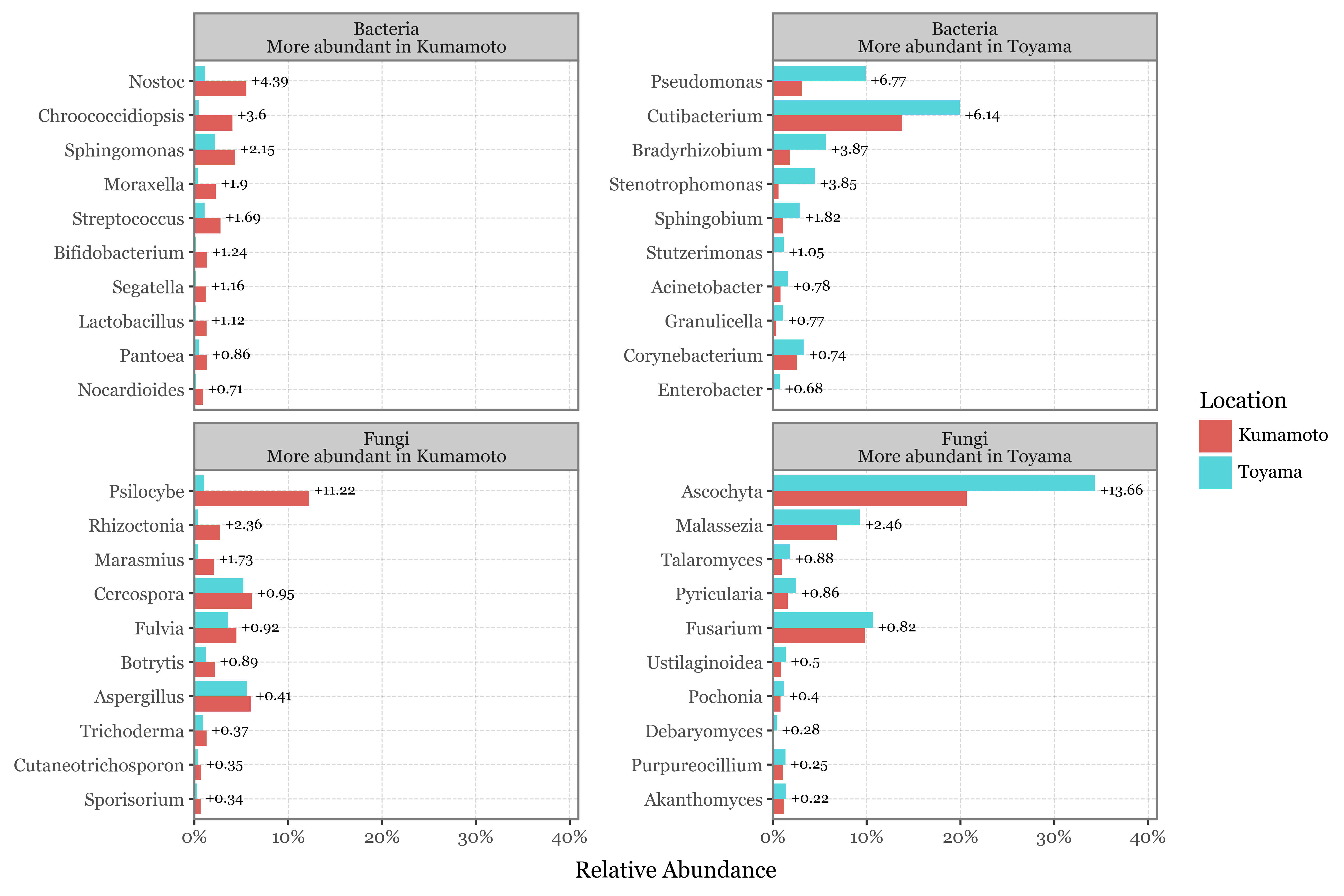
PM2.5 vs PM10 header
Show Code
headers_comp = (toyama_genera_pm10_stats
 .merge(toyama_genera_pm25_stats, on=['Kingdom', 'Genus'], suffixes=('_pm10', '_pm25'))
 .loc[lambda dd: (dd.relative_abundance_pm10 > .001) | (dd.relative_abundance_pm25 > .001)]
 .eval('ratio = relative_abundance_pm10 / relative_abundance_pm25')
 .assign(log_ratio=lambda dd: np.log2(dd['ratio']))
 .eval('diff = relative_abundance_pm10 - relative_abundance_pm25')
 .eval('selected = log_ratio.abs() > 3 or diff.abs() > .02')
 .eval('combined = log_ratio.abs() * diff.abs()')
 .eval('abs_diff = diff.abs()')
)

top_selected = headers_comp.sort_values('abs_diff', ascending=False).head(10).query('selected')


(headers_comp
.pipe(lambda dd: p9.ggplot(dd)
    + p9.aes('relative_abundance_pm10', 'relative_abundance_pm25')
    + p9.geom_point(p9.aes(color='Genus.isin(top_selected.Genus)'), stroke=0, size=1.5)
    + p9.scale_x_continuous(labels=percent_format(), limits=(-.001, .345))
    + p9.scale_y_continuous(labels=percent_format(), limits=(-.001, .345))
    + p9.geom_text(p9.aes(label='Genus'), size=7, data=top_selected, ha='left',
                    adjust_text={'expand': (1.5, 1.5), 'arrowprops': dict(arrowstyle='-', lw=0)})
    + p9.scale_color_manual({True: 'red', False: 'black'})
    + p9.guides(color=False)
    + p9.facet_wrap('Kingdom')
    + p9.geom_abline(intercept=0, slope=1, linetype='dashed')
    + p9.labs(x='Relative Abundance with PM$_{10}$ header', y='Relative Abundance with PM$_{2.5}$ header',
                color='Relative Abundance Difference', size='Log2(Ratio)')
    + p9.theme(figure_size=(6, 3),
               axis_text=p9.element_text(size=8),
               axis_title=p9.element_text(size=9),
    )
    )
)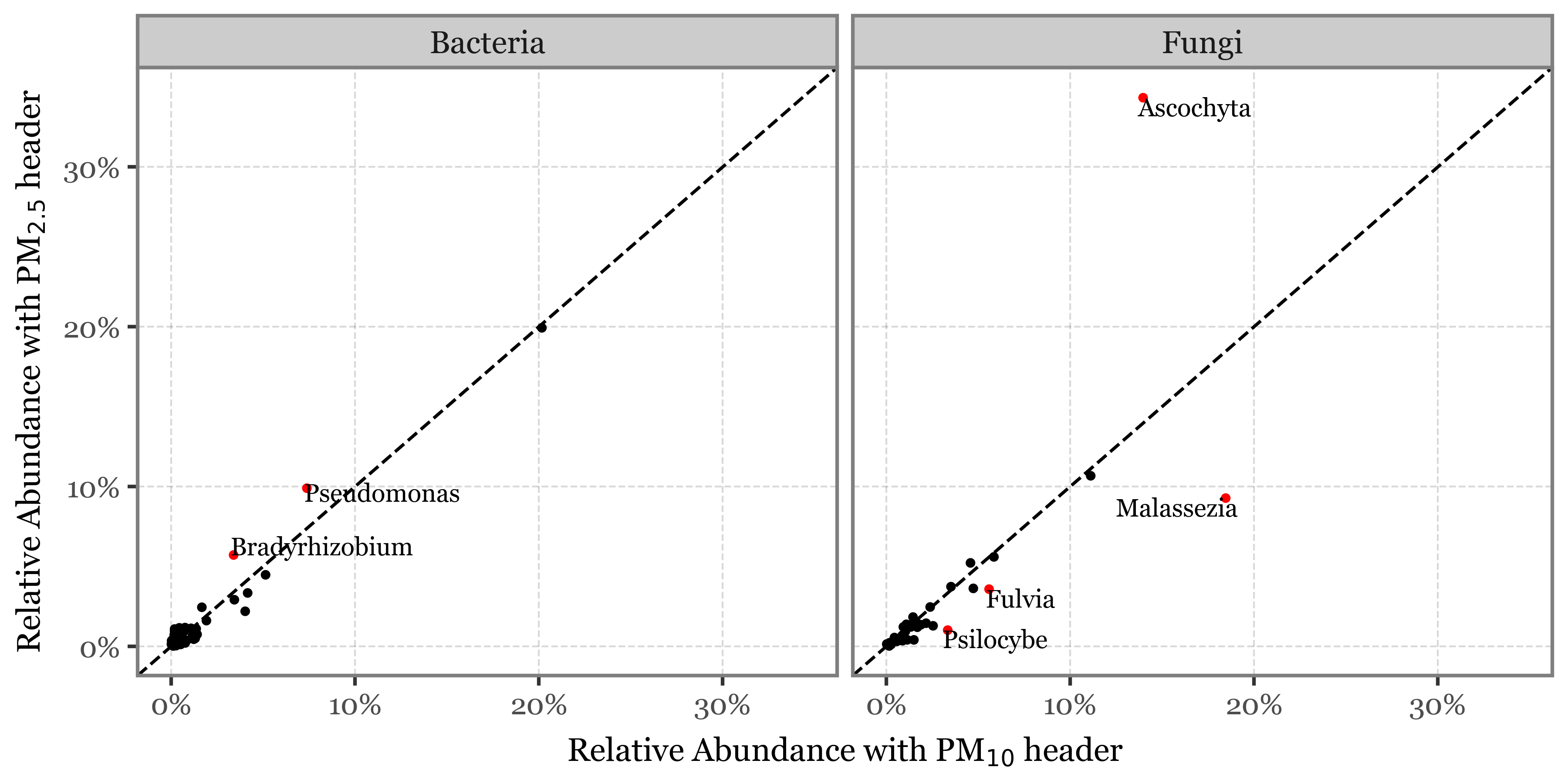
The differences are not as big as between Toyama and Kumamoto, but there are still some genera that show a big difference in relative abundance between the samples taken with the 2.5 and 10 um headers in Toyama. The full table:
Show Code
show(headers_comp
 .rename(columns={'relative_abundance_pm10': 'RA PM10', 'relative_abundance_pm25': 'RA PM2.5'})
 .sort_values('combined', ascending=False)
 [['Kingdom', 'Genus', 'RA PM10', 'RA PM2.5', 'abs_diff', 'ratio', 'log_ratio']]
 .style.format({'log_ratio': '{:.2f}', 'abs_diff': lambda x: f"{x * 100:.2f}", 'ratio': '{:.2f}',
                'RA PM10': '{:.2%}', 'RA PM2.5': '{:.2%}'})
 .hide(axis=0),
 buttons=['csv', 'colvis'], pageLength=20
)| Kingdom | Genus | RA PM10 | RA PM2.5 | abs_diff | ratio | log_ratio |
|---|---|---|---|---|---|---|
| Fungi | Ascochyta | 13.96% | 34.34% | 20.37 | 0.41 | -1.30 |
| Fungi | Malassezia | 18.46% | 9.27% | 9.19 | 1.99 | 0.99 |
| Fungi | Psilocybe | 3.33% | 1.01% | 2.32 | 3.31 | 1.72 |
| Bacteria | Granulicella | 0.18% | 1.08% | 0.90 | 0.16 | -2.61 |
| Fungi | Rhizoctonia | 1.49% | 0.40% | 1.09 | 3.75 | 1.91 |
| Bacteria | Terriglobus | 0.17% | 0.94% | 0.77 | 0.19 | -2.43 |
| Bacteria | Bradyrhizobium | 3.39% | 5.71% | 2.32 | 0.59 | -0.75 |
| Bacteria | Sphingomonas | 4.02% | 2.19% | 1.83 | 1.84 | 0.88 |
| Bacteria | Fibrella | 0.01% | 0.35% | 0.33 | 0.04 | -4.65 |
| Fungi | Fulvia | 5.58% | 3.57% | 2.01 | 1.56 | 0.64 |
| Fungi | Botrytis | 2.53% | 1.28% | 1.26 | 1.98 | 0.99 |
| Bacteria | Xanthomonas | 0.16% | 0.72% | 0.56 | 0.22 | -2.19 |
| Bacteria | Flavobacterium | 1.22% | 0.44% | 0.78 | 2.78 | 1.47 |
| Bacteria | Staphylococcus | 1.30% | 0.49% | 0.80 | 2.63 | 1.40 |
| Fungi | Cryptococcus | 1.13% | 0.40% | 0.73 | 2.82 | 1.49 |
| Bacteria | Pseudomonas | 7.37% | 9.89% | 2.52 | 0.75 | -0.42 |
| Bacteria | Rhodococcus | 0.75% | 0.21% | 0.55 | 3.66 | 1.87 |
| Bacteria | Nostoc | 0.43% | 1.15% | 0.72 | 0.38 | -1.41 |
| Bacteria | Caulobacter | 0.19% | 0.71% | 0.52 | 0.27 | -1.90 |
| Bacteria | Leuconostoc | 0.51% | 0.11% | 0.39 | 4.50 | 2.17 |
| Bacteria | Edaphobacter | 0.08% | 0.43% | 0.35 | 0.20 | -2.35 |
| Bacteria | Chroococcidiopsis | 0.10% | 0.45% | 0.35 | 0.23 | -2.13 |
| Fungi | Cutaneotrichosporon | 0.87% | 0.35% | 0.53 | 2.51 | 1.33 |
| Bacteria | Latilactobacillus | 0.26% | 0.04% | 0.22 | 6.71 | 2.75 |
| Bacteria | Enterobacter | 1.40% | 0.74% | 0.66 | 1.88 | 0.91 |
| Bacteria | Blastomonas | 0.01% | 0.14% | 0.13 | 0.05 | -4.42 |
| Bacteria | Spirosoma | 0.21% | 0.59% | 0.38 | 0.35 | -1.50 |
| Bacteria | Brevundimonas | 0.83% | 0.36% | 0.47 | 2.30 | 1.20 |
| Bacteria | Pelagibacterium | 0.01% | 0.13% | 0.12 | 0.07 | -3.92 |
| Bacteria | Streptomyces | 1.66% | 2.44% | 0.78 | 0.68 | -0.56 |
| Fungi | Zymoseptoria | 4.72% | 3.62% | 1.10 | 1.30 | 0.38 |
| Bacteria | Ensifer | 0.76% | 0.36% | 0.40 | 2.09 | 1.06 |
| Fungi | Marasmius | 0.78% | 0.38% | 0.40 | 2.06 | 1.04 |
| Fungi | Thermothielavioides | 2.15% | 1.44% | 0.71 | 1.49 | 0.58 |
| Fungi | Komagataella | 0.01% | 0.14% | 0.12 | 0.11 | -3.23 |
| Fungi | Zygotorulaspora | 0.15% | 0.02% | 0.13 | 8.12 | 3.02 |
| Bacteria | Pseudoxanthomonas | 0.66% | 0.31% | 0.35 | 2.11 | 1.08 |
| Bacteria | Brucella | 1.15% | 0.68% | 0.47 | 1.69 | 0.76 |
| Bacteria | Deinococcus | 0.07% | 0.25% | 0.19 | 0.27 | -1.88 |
| Bacteria | Brevibacterium | 0.22% | 0.50% | 0.28 | 0.43 | -1.20 |
| Bacteria | Moraxella | 0.73% | 0.38% | 0.35 | 1.93 | 0.95 |
| Bacteria | Paracoccus | 0.42% | 0.18% | 0.24 | 2.32 | 1.22 |
| Bacteria | Stutzerimonas | 0.74% | 1.17% | 0.42 | 0.64 | -0.65 |
| Bacteria | Kocuria | 0.28% | 0.10% | 0.18 | 2.81 | 1.49 |
| Bacteria | Enhydrobacter | 0.41% | 0.18% | 0.23 | 2.28 | 1.19 |
| Bacteria | Corynebacterium | 4.15% | 3.34% | 0.82 | 1.24 | 0.32 |
| Bacteria | Mycobacteroides | 0.07% | 0.22% | 0.15 | 0.31 | -1.70 |
| Fungi | Purpureocillium | 1.87% | 1.35% | 0.53 | 1.39 | 0.48 |
| Fungi | Neurospora | 1.68% | 1.19% | 0.49 | 1.41 | 0.50 |
| Bacteria | Escherichia | 0.19% | 0.06% | 0.14 | 3.33 | 1.74 |
| Bacteria | Roseomonas | 0.03% | 0.14% | 0.11 | 0.23 | -2.12 |
| Fungi | Sporisorium | 0.56% | 0.30% | 0.26 | 1.85 | 0.89 |
| Bacteria | Luteibacter | 0.12% | 0.02% | 0.09 | 5.26 | 2.39 |
| Bacteria | Mesorhizobium | 0.36% | 0.63% | 0.27 | 0.57 | -0.81 |
| Bacteria | Rhizorhabdus | 0.10% | 0.02% | 0.08 | 5.45 | 2.45 |
| Bacteria | Cronobacter | 0.14% | 0.04% | 0.10 | 3.82 | 1.93 |
| Bacteria | Polynucleobacter | 0.14% | 0.04% | 0.10 | 3.66 | 1.87 |
| Bacteria | Stieleria | 0.12% | 0.03% | 0.09 | 4.21 | 2.07 |
| Bacteria | Curtobacterium | 0.25% | 0.11% | 0.14 | 2.35 | 1.23 |
| Bacteria | Microlunatus | 0.05% | 0.15% | 0.10 | 0.31 | -1.68 |
| Bacteria | Ralstonia | 0.31% | 0.14% | 0.16 | 2.12 | 1.08 |
| Fungi | Kluyveromyces | 0.24% | 0.11% | 0.14 | 2.30 | 1.20 |
| Bacteria | Comamonas | 0.18% | 0.07% | 0.11 | 2.70 | 1.43 |
| Bacteria | Actinomyces | 0.29% | 0.14% | 0.15 | 2.06 | 1.04 |
| Bacteria | Gordonia | 0.46% | 0.70% | 0.24 | 0.65 | -0.61 |
| Bacteria | Pseudoalteromonas | 0.17% | 0.07% | 0.10 | 2.46 | 1.30 |
| Bacteria | Stenotrophomonas | 5.13% | 4.47% | 0.66 | 1.15 | 0.20 |
| Fungi | Talaromyces | 1.44% | 1.83% | 0.38 | 0.79 | -0.34 |
| Bacteria | Porphyromonas | 0.16% | 0.06% | 0.10 | 2.51 | 1.33 |
| Fungi | Scheffersomyces | 0.20% | 0.09% | 0.11 | 2.22 | 1.15 |
| Bacteria | Micrococcus | 0.13% | 0.04% | 0.08 | 2.88 | 1.53 |
| Bacteria | Mucilaginibacter | 0.09% | 0.21% | 0.11 | 0.46 | -1.12 |
| Fungi | Cercospora | 4.57% | 5.22% | 0.65 | 0.88 | -0.19 |
| Bacteria | Methylomonas | 0.10% | 0.03% | 0.07 | 3.28 | 1.71 |
| Bacteria | Sphingobium | 3.43% | 2.91% | 0.52 | 1.18 | 0.24 |
| Bacteria | Lactobacillus | 0.08% | 0.18% | 0.10 | 0.43 | -1.20 |
| Fungi | Debaryomyces | 0.62% | 0.42% | 0.21 | 1.49 | 0.58 |
| Fungi | Pochonia | 0.92% | 1.21% | 0.29 | 0.76 | -0.40 |
| Bacteria | Lawsonella | 0.30% | 0.17% | 0.13 | 1.79 | 0.84 |
| Bacteria | Rhizobium | 0.68% | 0.92% | 0.25 | 0.73 | -0.45 |
| Bacteria | Massilia | 0.28% | 0.16% | 0.12 | 1.78 | 0.83 |
| Bacteria | Mycolicibacterium | 0.63% | 0.44% | 0.19 | 1.44 | 0.52 |
| Fungi | Ustilaginoidea | 1.08% | 1.37% | 0.29 | 0.79 | -0.34 |
| Bacteria | Rothia | 0.18% | 0.09% | 0.09 | 2.01 | 1.01 |
| Bacteria | Actinoplanes | 0.04% | 0.11% | 0.07 | 0.40 | -1.33 |
| Bacteria | Neisseria | 0.25% | 0.14% | 0.11 | 1.77 | 0.82 |
| Fungi | Schizosaccharomyces | 0.05% | 0.12% | 0.07 | 0.42 | -1.25 |
| Fungi | Brettanomyces | 0.07% | 0.15% | 0.08 | 0.46 | -1.11 |
| Bacteria | Klebsiella | 0.08% | 0.17% | 0.08 | 0.50 | -1.01 |
| Bacteria | Chryseobacterium | 0.29% | 0.18% | 0.12 | 1.65 | 0.72 |
| Bacteria | Segatella | 0.05% | 0.12% | 0.07 | 0.43 | -1.22 |
| Bacteria | Streptococcus | 1.35% | 1.09% | 0.26 | 1.24 | 0.30 |
| Bacteria | Acinetobacter | 1.91% | 1.61% | 0.30 | 1.19 | 0.25 |
| Bacteria | Methylobacterium | 0.59% | 0.77% | 0.19 | 0.76 | -0.40 |
| Bacteria | Prevotella | 0.30% | 0.20% | 0.11 | 1.55 | 0.63 |
| Fungi | Yarrowia | 0.18% | 0.10% | 0.08 | 1.80 | 0.84 |
| Bacteria | Nocardia | 0.07% | 0.14% | 0.07 | 0.53 | -0.93 |
| Fungi | Penicillium | 0.86% | 0.68% | 0.18 | 1.26 | 0.34 |
| Bacteria | Agromyces | 0.12% | 0.06% | 0.06 | 2.02 | 1.02 |
| Fungi | Akanthomyces | 1.68% | 1.43% | 0.25 | 1.17 | 0.23 |
| Bacteria | Amycolatopsis | 0.28% | 0.19% | 0.09 | 1.49 | 0.58 |
| Bacteria | Leptolyngbya | 0.05% | 0.10% | 0.05 | 0.49 | -1.03 |
| Bacteria | Cellulomonas | 0.14% | 0.07% | 0.06 | 1.82 | 0.87 |
| Bacteria | Bosea | 0.18% | 0.11% | 0.07 | 1.65 | 0.72 |
| Bacteria | Bacteroides | 0.19% | 0.12% | 0.07 | 1.59 | 0.66 |
| Bacteria | Achromobacter | 0.14% | 0.08% | 0.06 | 1.74 | 0.80 |
| Fungi | Ogataea | 0.11% | 0.06% | 0.05 | 1.88 | 0.91 |
| Bacteria | Bacillus | 0.38% | 0.28% | 0.10 | 1.36 | 0.45 |
| Fungi | Sugiyamaella | 0.07% | 0.12% | 0.05 | 0.56 | -0.83 |
| Bacteria | Brevibacillus | 0.11% | 0.06% | 0.05 | 1.82 | 0.87 |
| Fungi | Eremothecium | 0.19% | 0.12% | 0.07 | 1.55 | 0.63 |
| Bacteria | Aureimonas | 0.11% | 0.06% | 0.05 | 1.81 | 0.86 |
| Bacteria | Clostridium | 0.21% | 0.14% | 0.07 | 1.49 | 0.57 |
| Fungi | Puccinia | 0.43% | 0.54% | 0.11 | 0.80 | -0.33 |
| Bacteria | Devosia | 0.13% | 0.20% | 0.06 | 0.68 | -0.56 |
| Fungi | Tetrapisispora | 0.17% | 0.11% | 0.06 | 1.53 | 0.61 |
| Bacteria | Lysobacter | 0.16% | 0.11% | 0.06 | 1.51 | 0.60 |
| Bacteria | Serratia | 0.07% | 0.11% | 0.04 | 0.61 | -0.71 |
| Bacteria | Cupriavidus | 0.21% | 0.28% | 0.07 | 0.74 | -0.43 |
| Bacteria | Erythrobacter | 0.06% | 0.10% | 0.04 | 0.60 | -0.73 |
| Fungi | Fusarium | 11.11% | 10.67% | 0.44 | 1.04 | 0.06 |
| Bacteria | Nordella | 0.11% | 0.07% | 0.04 | 1.57 | 0.65 |
| Fungi | Saccharomyces | 0.16% | 0.22% | 0.05 | 0.75 | -0.41 |
| Fungi | Colletotrichum | 3.51% | 3.73% | 0.22 | 0.94 | -0.09 |
| Bacteria | Aeromonas | 0.15% | 0.20% | 0.05 | 0.76 | -0.39 |
| Bacteria | Bifidobacterium | 0.16% | 0.12% | 0.04 | 1.35 | 0.43 |
| Bacteria | Mycobacterium | 0.25% | 0.31% | 0.06 | 0.82 | -0.29 |
| Bacteria | Micromonospora | 0.24% | 0.19% | 0.05 | 1.26 | 0.34 |
| Bacteria | Shewanella | 0.46% | 0.54% | 0.08 | 0.86 | -0.22 |
| Fungi | Aspergillus | 5.85% | 5.59% | 0.25 | 1.05 | 0.06 |
| Fungi | Drechmeria | 1.32% | 1.21% | 0.12 | 1.10 | 0.13 |
| Fungi | Trichoderma | 1.03% | 0.93% | 0.10 | 1.11 | 0.14 |
| Bacteria | Novosphingobium | 0.33% | 0.28% | 0.05 | 1.19 | 0.25 |
| Bacteria | Pedobacter | 0.08% | 0.11% | 0.03 | 0.74 | -0.44 |
| Bacteria | Bordetella | 0.20% | 0.16% | 0.04 | 1.25 | 0.32 |
| Bacteria | Shinella | 0.17% | 0.13% | 0.03 | 1.25 | 0.33 |
| Bacteria | Sphingobacterium | 0.08% | 0.10% | 0.03 | 0.75 | -0.41 |
| Fungi | Ustilago | 0.29% | 0.25% | 0.04 | 1.16 | 0.21 |
| Bacteria | Citrobacter | 0.09% | 0.11% | 0.02 | 0.80 | -0.32 |
| Bacteria | Sphingopyxis | 0.19% | 0.23% | 0.03 | 0.86 | -0.22 |
| Bacteria | Agrobacterium | 0.37% | 0.32% | 0.04 | 1.13 | 0.17 |
| Bacteria | Variovorax | 0.36% | 0.33% | 0.04 | 1.12 | 0.16 |
| Bacteria | Halomonas | 0.13% | 0.11% | 0.02 | 1.20 | 0.27 |
| Bacteria | Paraburkholderia | 0.22% | 0.20% | 0.02 | 1.13 | 0.17 |
| Fungi | Thermothelomyces | 1.49% | 1.55% | 0.06 | 0.96 | -0.06 |
| Bacteria | Paenibacillus | 0.34% | 0.37% | 0.03 | 0.92 | -0.12 |
| Bacteria | Cutibacterium | 20.16% | 19.93% | 0.23 | 1.01 | 0.02 |
| Fungi | Pyricularia | 2.38% | 2.46% | 0.08 | 0.97 | -0.05 |
| Bacteria | Hymenobacter | 1.07% | 1.12% | 0.05 | 0.96 | -0.07 |
| Bacteria | Lacipirellula | 0.23% | 0.21% | 0.02 | 1.10 | 0.14 |
| Bacteria | Sinorhizobium | 0.11% | 0.13% | 0.02 | 0.88 | -0.18 |
| Bacteria | Arthrobacter | 0.26% | 0.24% | 0.02 | 1.09 | 0.12 |
| Bacteria | Nocardioides | 0.20% | 0.19% | 0.01 | 1.07 | 0.10 |
| Fungi | Candida | 0.21% | 0.22% | 0.01 | 0.94 | -0.09 |
| Bacteria | Sneathiella | 0.14% | 0.13% | 0.01 | 1.07 | 0.10 |
| Bacteria | Azospirillum | 0.13% | 0.12% | 0.01 | 1.05 | 0.07 |
| Bacteria | Burkholderia | 0.35% | 0.34% | 0.01 | 1.03 | 0.04 |
| Bacteria | Roseateles | 0.12% | 0.11% | 0.01 | 1.05 | 0.07 |
| Bacteria | Vibrio | 0.38% | 0.37% | 0.01 | 1.02 | 0.03 |
| Bacteria | Pantoea | 0.48% | 0.48% | 0.01 | 0.99 | -0.02 |
| Bacteria | Microbacterium | 0.50% | 0.50% | 0.00 | 1.01 | 0.01 |
Show Code
(headers_comp
 .assign(direction=lambda dd: np.where(dd['ratio'] > 1, 'PM10', 'PM2.5'))
 .groupby(['direction', 'Kingdom'],  as_index=False)
 .apply(lambda dd: dd.sort_values('abs_diff', ascending=False).head(10))
 [['Kingdom', 'Genus', 'direction', 'relative_abundance_pm10', 'relative_abundance_pm25', 'abs_diff']]
 .melt(['Kingdom', 'Genus', 'direction', 'abs_diff'], var_name='location', value_name='relative_abundance')
 .assign(location=lambda dd: dd.location.str.split('_').str[-1].str.upper())
 .replace({'PM25': 'PM2.5'})
 .eval('selected= direction == location')
 .replace({'direction': {'PM10': 'More abundant in PM$_{10}$', 'PM2.5': 'More abundant in PM$_{2.5}$'}})
 .pipe(lambda dd: p9.ggplot(dd)
    + p9.aes('reorder(Genus, abs_diff)', 'relative_abundance', fill='location')
    + p9.geom_col(position='dodge')
    + p9.geom_text(p9.aes(label='"+" + (abs_diff * 100).round(2).astype(str)'), size=7, ha='left', nudge_y=.005,
                   data=dd.query('selected'))
    + p9.coord_flip()
    + p9.scale_y_continuous(labels=percent_format(), expand=(0, 0, .175, 0))
    + p9.labs(x='', y='Relative Abundance', fill='Location')
    + p9.facet_wrap(['Kingdom', 'direction'], scales='free_y')
    + p9.theme(figure_size=(9, 6))

 )

)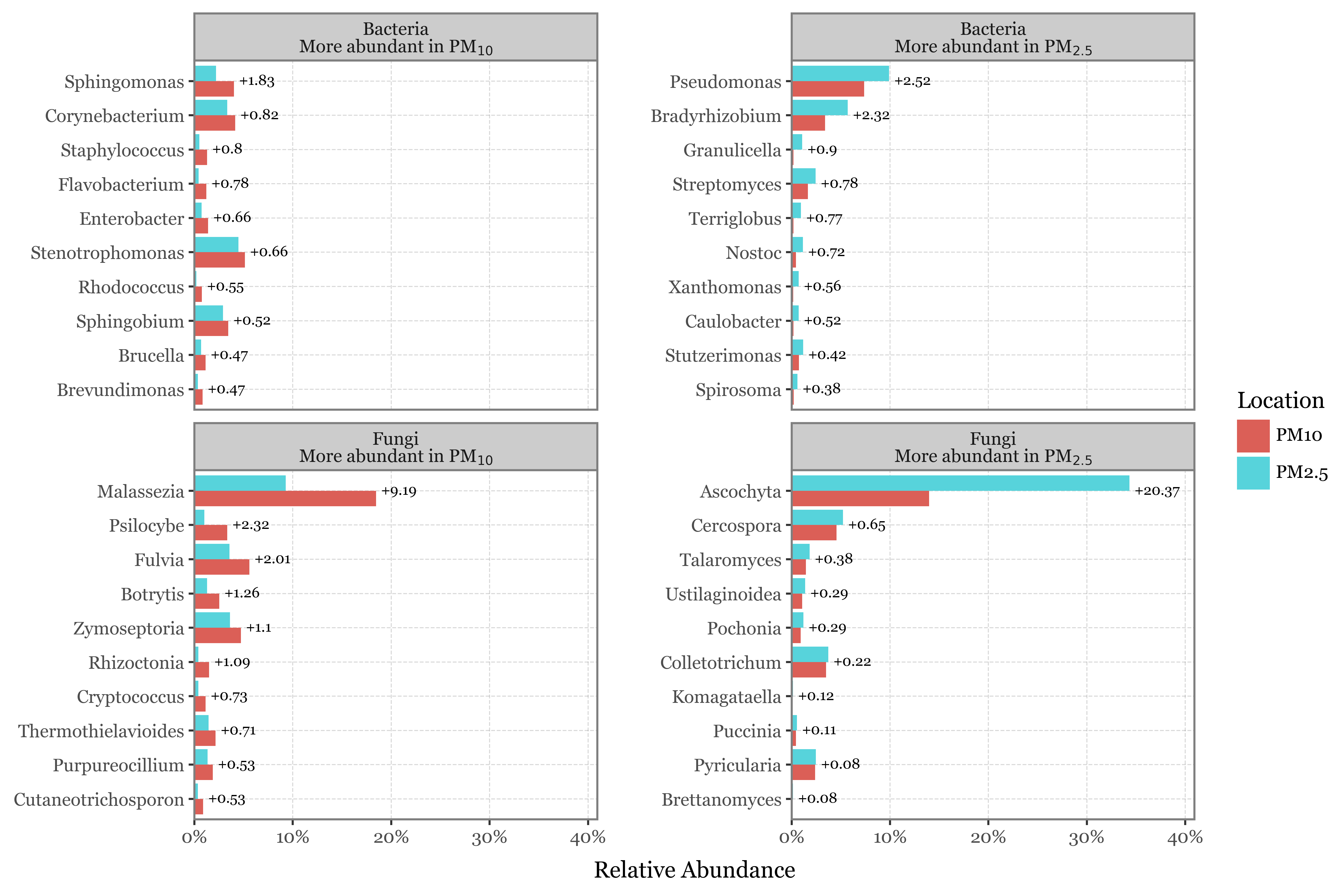
Association with Kawasaki Disease
To check the association of the presence and abundance of different microbial taxa with the incidence of Kawasaki Disease, we will use the data from the nationwide surveys of KD in Japan.
Visualizing the experimental setup
Matching the data from the prefectural KD incidence to the daily and weekly samples is not trivial, since the frequency of the samples is not homogeneous, the coverage is not complete for the whole 2017-2018 period, and we don’t really have a proper proxy for the absolute abundance of the different taxa in the environment as a function of time.
Nevertheless, this is how the timeline of the samples with respect to the KD incidence in the prefecture, the section and the whole of Japan for both Kumamoto and Toyama looks like:
Data preparation for regional KD data
kd_df = pd.read_csv('../../kd-spatial-ts/data/kawasaki_full_2020.csv')

kyushu_prefectures = [f'JP-{str(i).zfill(2)}' for i in range(40, 47)]
chubu_prefectures = [f'JP-{str(i).zfill(2)}' for i in range(15, 24)]

kd_japan = (kd_df
 .assign(date_visit=lambda dd: pd.to_datetime(dd.date_visit))
 .assign(date_onset=lambda dd: dd.date_visit - pd.to_timedelta(dd.dayvisit - 1, unit='D'))
 .assign(cases=1)
 [['date_onset', 'date_visit', 'cases']]
 .melt('cases', value_name='date')
 .groupby('variable')
 .apply(lambda dd: dd.set_index('date').resample('D')['cases'].sum())
 .reset_index()
 .groupby('variable')
 .apply(lambda dd: dd.assign(rolling_cases=dd['cases'].rolling(7, center=True).mean()))
 .query('variable=="date_onset"')
 .replace({'variable': {'date_onset': 'Registered Onsets', 'date_visit': 'Hospital Admissions'}})
 .assign(region='Japan')
)

kd_kyushu = (kd_df
 .query('prefecture_code in @kyushu_prefectures')
 .assign(date_visit=lambda dd: pd.to_datetime(dd.date_visit))
 .assign(date_onset=lambda dd: dd.date_visit - pd.to_timedelta(dd.dayvisit - 1, unit='D'))
 .assign(cases=1)
 [['date_onset', 'date_visit', 'cases']]
 .melt('cases', value_name='date')
 .groupby('variable')
 .apply(lambda dd: dd.set_index('date').resample('D')['cases'].sum())
 .reset_index()
 .groupby('variable')
 .apply(lambda dd: dd.assign(rolling_cases=dd['cases'].rolling(7, center=True).mean()))
 .query('variable=="date_onset"')
 .replace({'variable': {'date_onset': 'Registered Onsets', 'date_visit': 'Hospital Admissions'}})
 .assign(region='Kyushu')
)

kd_chubu = (kd_df
    .query('prefecture_code in @chubu_prefectures')
    .assign(date_visit=lambda dd: pd.to_datetime(dd.date_visit))
    .assign(date_onset=lambda dd: dd.date_visit - pd.to_timedelta(dd.dayvisit - 1, unit='D'))
    .assign(cases=1)
    [['date_onset', 'date_visit', 'cases']]
    .melt('cases', value_name='date')
    .groupby('variable')
    .apply(lambda dd: dd.set_index('date').resample('D')['cases'].sum())
    .reset_index()
    .groupby('variable')
    .apply(lambda dd: dd.assign(rolling_cases=dd['cases'].rolling(7, center=True).mean()))
    .query('variable=="date_onset"')
    .replace({'variable': {'date_onset': 'Registered Onsets', 'date_visit': 'Hospital Admissions'}})
    .assign(region='Chubu')
    )

kd_kumamoto = (kd_df
    .query('prefecture_code=="JP-43"')
    .assign(date_visit=lambda dd: pd.to_datetime(dd.date_visit))
    .assign(date_onset=lambda dd: dd.date_visit - pd.to_timedelta(dd.dayvisit - 1, unit='D'))
    .assign(cases=1)
    [['date_onset', 'date_visit', 'cases']]
    .melt('cases', value_name='date')
    .groupby('variable')
    .apply(lambda dd: dd.set_index('date').resample('D')['cases'].sum())
    .reset_index()
    .groupby('variable')
    .apply(lambda dd: dd.assign(rolling_cases=dd['cases'].rolling(7, center=True).mean()))
    .query('variable=="date_onset"')
    .replace({'variable': {'date_onset': 'Registered Onsets', 'date_visit': 'Hospital Admissions'}})
    .assign(region='Kumamoto')
    )

kd_toyama = (kd_df
    .query('prefecture_code=="JP-16"')
    .assign(date_visit=lambda dd: pd.to_datetime(dd.date_visit))
    .assign(date_onset=lambda dd: dd.date_visit - pd.to_timedelta(dd.dayvisit - 1, unit='D'))
    .assign(cases=1)
    [['date_onset', 'date_visit', 'cases']]
    .melt('cases', value_name='date')
    .groupby('variable')
    .apply(lambda dd: dd.set_index('date').resample('D')['cases'].sum())
    .reset_index()
    .groupby('variable')
    .apply(lambda dd: dd.assign(rolling_cases=dd['cases'].rolling(7, center=True).mean()))
    .query('variable=="date_onset"')
    .replace({'variable': {'date_onset': 'Registered Onsets', 'date_visit': 'Hospital Admissions'}})
    .assign(region='Toyama')
    )

japan_shape = japan_shape.assign(prefecture_code=lambda dd: 'JP-' + dd['ADM1_PCODE'].str[2:])
Show Code
(japan_shape
 .pipe(lambda dd: p9.ggplot(dd)
       + p9.geom_map(alpha=.1, size=.3)
       + p9.geom_map(japan_shape.query('ADM1_PCODE=="JP43"'), fill='red', size=.3)
       + p9.geom_map(japan_shape.query('prefecture_code in @kyushu_prefectures'), fill='salmon', size=.3, alpha=.7)
       + p9.xlim(129, 145)
       + p9.ylim(30, None)
       + p9.theme_void()
       + p9.theme(figure_size=(5.5, 6),
                  # plot_background=p9.element_rect(fill='white')
                  )
       )
)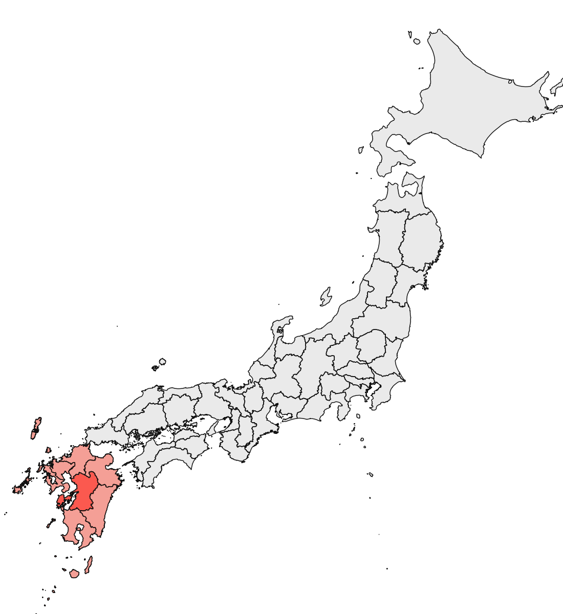
Show Code
(pd.concat([kd_japan, kd_kyushu, kd_kumamoto])
 .assign(region=lambda dd: pd.Categorical(dd.region, categories=['Japan', 'Kyushu', 'Kumamoto']))
 .query('"2017-05" <= date <= "2018-07"')
  .assign(date=lambda dd: pd.to_datetime(dd.date))
 .pipe(lambda dd: p9.ggplot(dd)
       + p9.aes(x='date', y='cases')
       + p9.geom_rect(p9.aes(xmin='start_date', xmax='end_date', ymin=-np.inf, ymax=np.inf),
                       fill='skyblue', alpha=.5, color='black', linetype='dashed',
                      size=.1,
                       data=kumamoto_samples, inherit_aes=False)
       + p9.geom_line()
       + p9.geom_line(p9.aes(y='rolling_cases'), color='red')
       + p9.scale_x_datetime(date_breaks='1 months', date_labels='%b %Y', expand=(0.01, 0, 0, 0))
       + p9.labs(x='', y='KD cases', color='', title='Timing of Kumamoto samples with Kawasaki Disease cases')
       + p9.facet_wrap('~region', scales='free_y', ncol=1)
       + p9.theme(
           axis_text_x=p9.element_text(angle=45),
           axis_text=p9.element_text(size=7),
           legend_position='top',
           figure_size=(5, 3.5),
           plot_background=p9.element_blank(),
           plot_title=p9.element_text(size=9)
       )
 )
)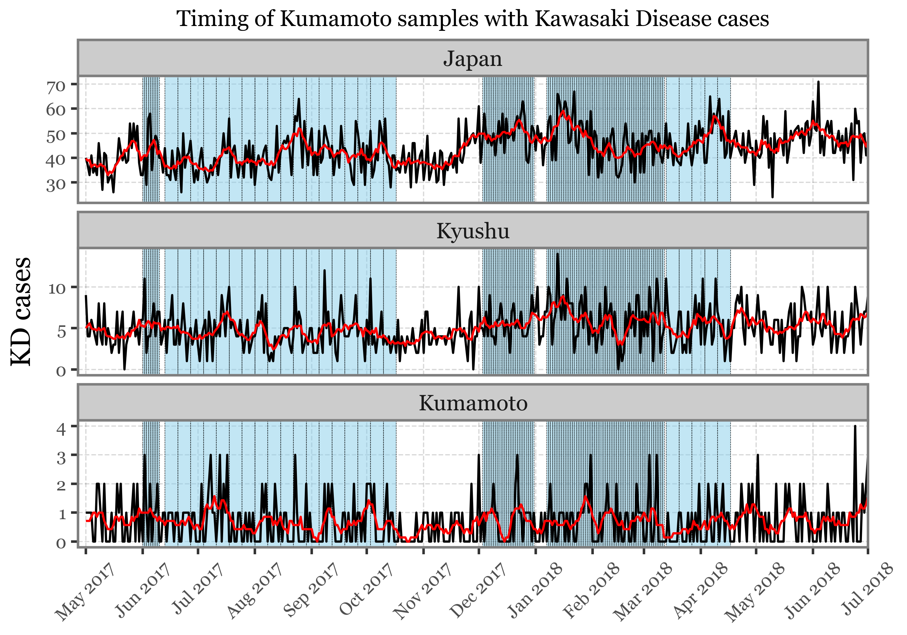
Show Code
(japan_shape
 .pipe(lambda dd: p9.ggplot(dd)
       + p9.geom_map(alpha=.1, size=.3)
       + p9.geom_map(japan_shape.query('ADM1_PCODE=="JP16"'), fill='red', size=.3)
       + p9.geom_map(japan_shape.query('prefecture_code in @chubu_prefectures'), fill='salmon', size=.3, alpha=.7)
       + p9.xlim(129, 145)
       + p9.ylim(30, None)
       + p9.theme_void()
       + p9.theme(figure_size=(5.5, 6),
                  )
       )
)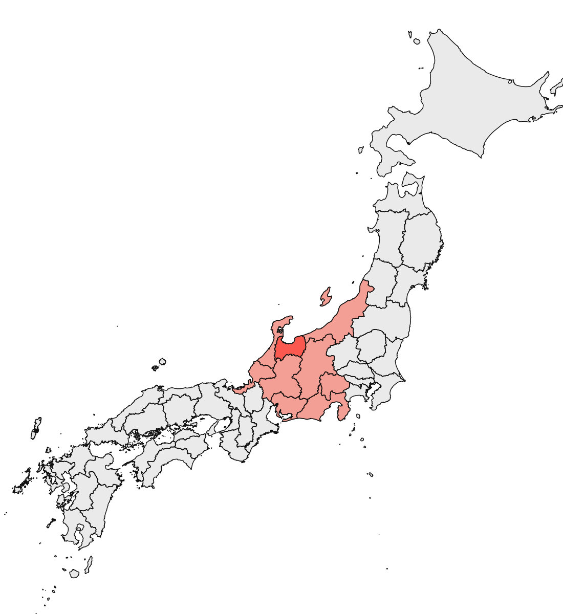
Show Code
(pd.concat([kd_japan, kd_chubu, kd_toyama])
 .assign(region=lambda dd: pd.Categorical(dd.region, categories=['Japan', 'Chubu', 'Toyama']))
 .query('"2017-05" <= date <= "2018-07"')
  .assign(date=lambda dd: pd.to_datetime(dd.date))
 .pipe(lambda dd: p9.ggplot(dd)
       + p9.aes(x='date', y='cases')
       + p9.geom_rect(p9.aes(xmin='start_date', xmax='end_date', ymin=-np.inf, ymax=np.inf, fill='header'),
                      alpha=.5, color='black', linetype='dashed',
                      size=.1, data=samples_info.assign(end_date=lambda dd: dd.end_dt.dt.date), inherit_aes=False)
       + p9.geom_line()
       + p9.geom_line(p9.aes(y='rolling_cases'), color='red')
       + p9.scale_x_datetime(date_breaks='1 months', date_labels='%b %Y', expand=(0.01, 0, 0, 0))
       + p9.labs(x='', y='KD cases', color='', fill='',
                 title='Timing of Toyama samples with Kawasaki Disease cases')
       + p9.facet_wrap('~region', scales='free_y', ncol=1)
       + p9.theme(
           axis_text_x=p9.element_text(angle=45),
           axis_text=p9.element_text(size=7),
           figure_size=(5.5, 3.5),
           legend_key_size=8,
           plot_background=p9.element_blank(),
           plot_title=p9.element_text(size=9)
       )
 )
)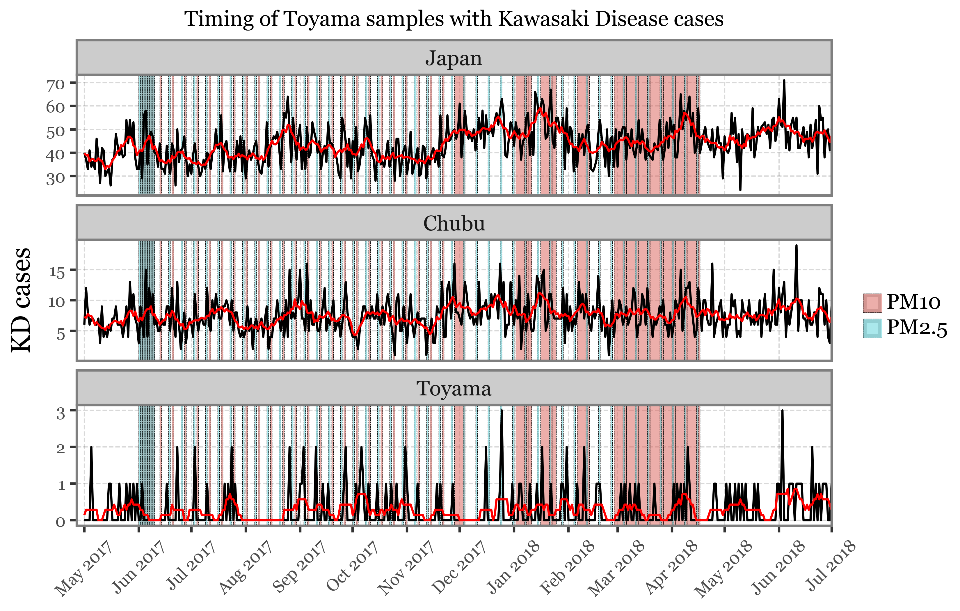
Total microbial load vs KD incidence
The standard method for quantifying the total biomass present in air samples involves using the DNA yield or the DNA yield normalized by the volume of air filtered. However, this approach encounters two different problems for our samples:
In the samples from Toyama, the weekly samples, which have filtered the most air by a good margin, show similar yields of DNA to the daily ones, but lower DNA yields when normalizing by the volume filtered. This could be due to DNA degradation in the filter after prolonged exposure, but if that is the case, what is clear is that we end up underestimating the total biomass of the samples with longer sampling time.
In the case of Kumamoto, we have the very opposite problem: the volume-normalized DNA yield is higher than the yield of the daily samples. It could simply be that the time period of the weekly samples was a season of higher aerobiomass, but it is in any case quite surprising that we find this contradiction between the different locations.
Additionally, we observed that the total reads per sample in Kraken show no association whatsoever with the DNA yield, which is our closest measure of the total biomass of the samples. Therefore, the total reads cannot be reliably used as a proxy of abundance in the enviroment either.
In any case, and despite my skepticism, we will take a look at the data.
We will begin by examining the case of Kumamoto, where all the headers are comparable.
To conduct a straightforward yet fair analysis, we will use the normalized DNA yield of the samples as a proxy for the total biomass. We will then correlate this with the average incidence of KD in the prefecture, section, or entire Japan for the sampling days (including only days with samples starting in the morning) plus three days following the sampling, similar to the methodology we used in (Rodó et al. 2023).
The four variables and series we will cross-correlate look as follows once prepared:
(Note that we use the daily average for the period of the samples plus three days, as some samples span an uneven number of days):
Show Code
kumamoto_comp_ts = (kumamoto_calendar
 .query('sample_id.notna()')
 .assign(start_hour=lambda dd: np.where(dd.date == dd.start_date, dd.start_dt.dt.hour, 0))
 .query('start_hour < 12')
 .groupby('sample_id')
 .apply(lambda dd: dd
        .query('date==date.max()')
        .assign(date=[pd.date_range(dd.date.min(), dd.date.max() + pd.to_timedelta(3, unit='D'))])
        ['date'])
 .reset_index()
 .explode('date')
 .merge(kd_japan[['date', 'cases']].rename(columns={'cases': 'cases_japan'}), how='left')
 .merge(kd_kyushu[['date', 'cases']].rename(columns={'cases': 'cases_kyushu'}), how='left')
 .merge(kd_kumamoto[['date', 'cases']].rename(columns={'cases': 'cases_kumamoto'}), how='left')
 .merge(kumamoto_samples)
 .merge(pacbio_metrics, on=['sample_id', 'header'])
 .assign(norm_dna=lambda dd: dd.dna_total / dd['volume'])
 .groupby('sample_id')
 .agg({'cases_kumamoto': 'mean', 'cases_kyushu': 'mean', 'cases_japan': 'mean', 'norm_dna': 'mean'})
 )

(kumamoto_comp_ts
 .reset_index()
 .melt('sample_id')
 .replace({'variable': {'cases_japan': '(b) KD cases in Japan',
                        'cases_kyushu': '(c) KD cases in Kyushu',
                        'cases_kumamoto': '(d) KD cases in Kumamoto',
                         'norm_dna': '(a) DNA yield (ng/m3)'}})
 .pipe(lambda dd: p9.ggplot(dd)
       + p9.aes(x='sample_id', y='value')
       + p9.geom_col(p9.aes(alpha='variable'))
       + p9.geom_line(p9.aes(group='variable'))
       + p9.scale_alpha_manual([1, 0, 0, 0])
       + p9.scale_x_discrete(breaks=sorted(dd.sample_id.unique())[::3])
       + p9.facet_wrap('~variable', scales='free_y', ncol=1)
       + p9.guides(color=False, alpha=False)
       + p9.labs(x='', y='')
       + p9.theme(figure_size=(6, 4),
                  axis_text_x=p9.element_text(angle=90, size=7, family='monospace'),
       )
       )
 )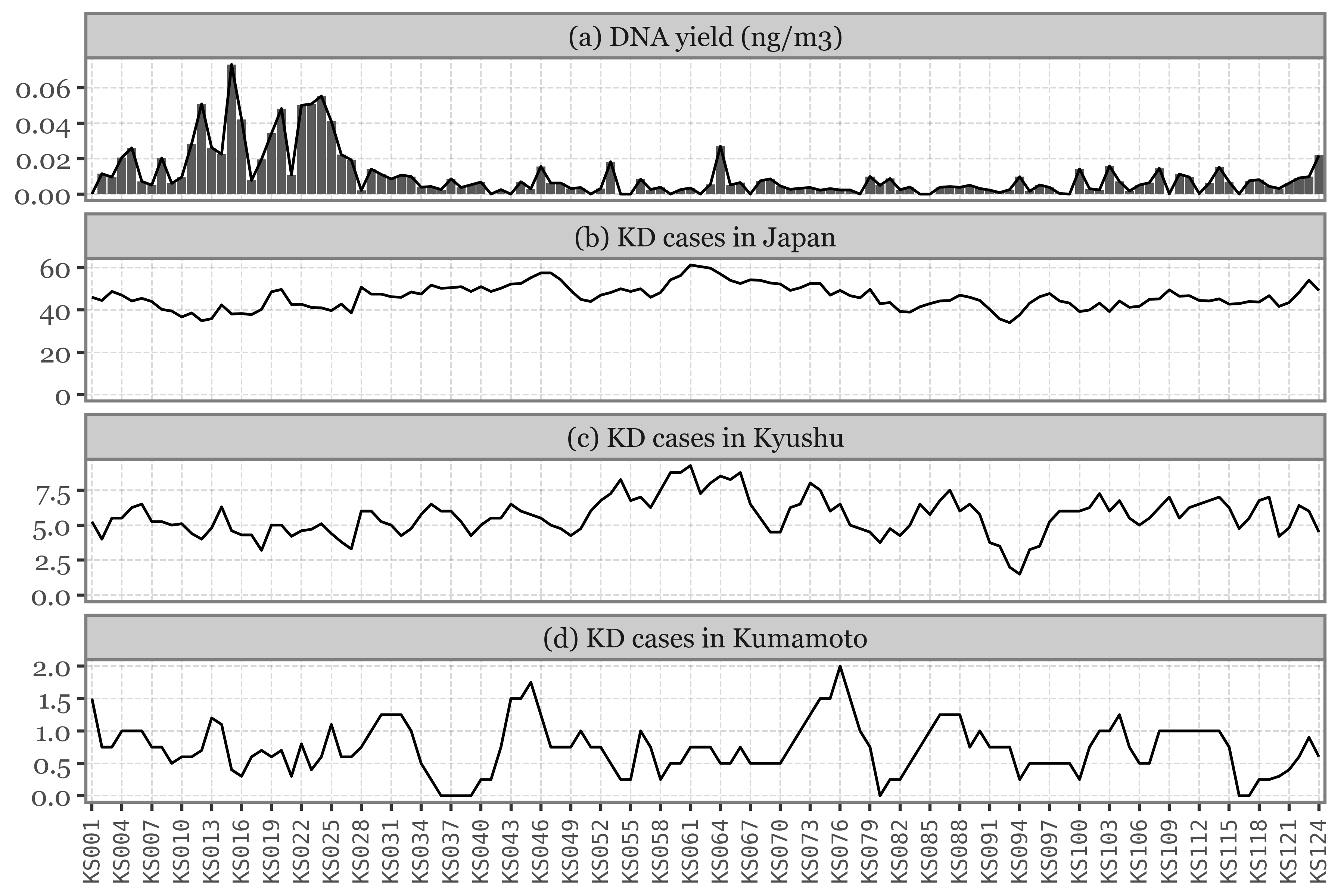
The correlation of the first series (a) with the other three is then:
Show Code
from scipy.stats import spearmanr
(kumamoto_comp_ts
 .corr(method=lambda x, y: spearmanr(x, y)[0])
 .loc['norm_dna']
 .iloc[:-1]
 .rename("Spearman's r")
 .reset_index()
 .assign(p_value=kumamoto_comp_ts.corr(method=lambda x, y: spearmanr(x, y)[1])
         .loc['norm_dna'].iloc[:-1].to_list())
 .replace({'index': {'cases_japan': 'KD cases in Japan',
                          'cases_kyushu': 'KD cases in Kyushu',
                          'cases_kumamoto': 'KD cases in Kumamoto'}})

)| index | Spearman's r | p_value |
|---|---|---|
|
Loading ITables v2.1.4 from the init_notebook_mode cell...
(need help?) |
The series are either non-correlated or negatively so, thus we can’t find any association between the total biomass in the air and the incidence of KD in Kumamoto/Kyushu/Japan.
We know that we might be overestimating the total biomass in the samples with longer sampling times, so we will now repeat the analysis but only for the samples that have a comparable sampling time, which are the daily samples. Dropping those samples, the newly prepared series are:
Show Code
kumamoto_comp_ts_daily = (kumamoto_calendar
 .query('sample_id.notna()')
 .assign(start_hour=lambda dd: np.where(dd.date == dd.start_date, dd.start_dt.dt.hour, 0))
 .query('start_hour < 12')
 .groupby('sample_id')
 .apply(lambda dd: dd
        .query('date==date.max()')
        .assign(date=[pd.date_range(dd.date.min(), dd.date.max() + pd.to_timedelta(3, unit='D'))])
        ['date'])
 .reset_index()
 .explode('date')
 .merge(kd_japan[['date', 'cases']].rename(columns={'cases': 'cases_japan'}), how='left')
 .merge(kd_kyushu[['date', 'cases']].rename(columns={'cases': 'cases_kyushu'}), how='left')
 .merge(kd_kumamoto[['date', 'cases']].rename(columns={'cases': 'cases_kumamoto'}), how='left')
 .merge(kumamoto_samples)
 .query('duration < 25')
 .merge(pacbio_metrics, on=['sample_id', 'header'])
 .assign(norm_dna=lambda dd: dd.dna_total / dd['volume'])
 .groupby('sample_id')
 .agg({'cases_kumamoto': 'mean', 'cases_kyushu': 'mean', 'cases_japan': 'mean', 'norm_dna': 'mean'})
 )

(kumamoto_comp_ts_daily
 .reset_index()
 .melt('sample_id')
 .replace({'variable': {'cases_japan': '(b) KD cases in Japan',
                        'cases_kyushu': '(c) KD cases in Kyushu',
                        'cases_kumamoto': '(d) KD cases in Kumamoto',
                         'norm_dna': '(a) DNA yield (ng/m3)'}})
 .pipe(lambda dd: p9.ggplot(dd)
       + p9.aes(x='sample_id', y='value')
       + p9.geom_col(p9.aes(alpha='variable'))
       + p9.geom_line(p9.aes(group='variable'))
       + p9.scale_alpha_manual([1, 0, 0, 0])
       + p9.scale_x_discrete(breaks=sorted(dd.sample_id.unique())[::3])
       + p9.facet_wrap('~variable', scales='free_y', ncol=1)
       + p9.guides(color=False, alpha=False)
       + p9.labs(x='', y='')
       + p9.theme(figure_size=(6, 4),
                  axis_text_x=p9.element_text(angle=90, size=7, family='monospace'),
       )
       )
 )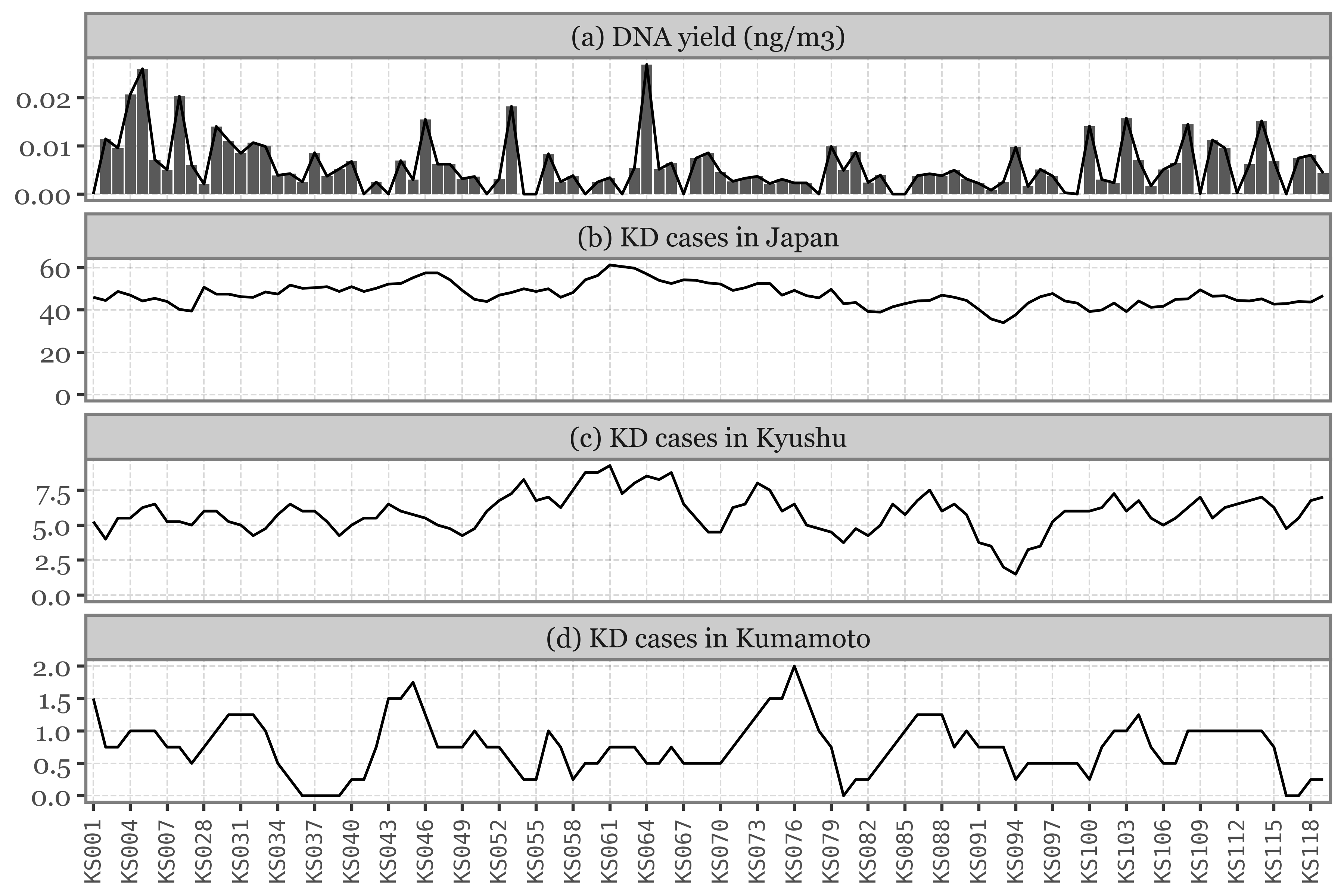
Show Code
(kumamoto_comp_ts_daily
 .corr(method=lambda x, y: spearmanr(x, y)[0])
 .loc['norm_dna']
 .iloc[:-1]
 .rename("Spearman's r")
 .reset_index()
 .assign(p_value=kumamoto_comp_ts_daily.corr(method=lambda x, y: spearmanr(x, y)[1])
         .loc['norm_dna'].iloc[:-1].to_list())
 .replace({'index': {'cases_japan': 'KD cases in Japan',
                          'cases_kyushu': 'KD cases in Kyushu',
                          'cases_kumamoto': 'KD cases in Kumamoto'}})

)| index | Spearman's r | p_value |
|---|---|---|
|
Loading ITables v2.1.4 from the init_notebook_mode cell...
(need help?) |
Some small changes, but no meaningful changes in the correlation values. Our previous conclusion still stands.
Let’s now do the same analysis for Toyama, where the headers are different, so we will be splitting the DNA yield by header type too.
Show Code
pacbio_toyama = (pacbio_metrics.query('sample_id.str.startswith("TS")')
 .assign(sample_id=lambda dd: 'TS' + dd.sample_id.str.split('.').str[0].str[2:].str.zfill(2))
)

toyama_comp_ts = (toyama_calendar
 .query('sample_id.notna()')
 .assign(start_hour=lambda dd: np.where(dd.date == dd.start_date, dd.start_dt.dt.hour, 0))
 .query('start_hour < 12')
 .groupby('sample_id')
 .apply(lambda dd: dd
        .query('date==date.max()')
        .assign(date=[pd.date_range(dd.date.min(), dd.date.max() + pd.to_timedelta(3, unit='D'))])
        ['date'])
 .reset_index()
 .explode('date')
 .merge(samples_info[['sample_id', 'header', 'volume']])
 .assign(sample_id=lambda dd: 'TS' + dd.sample_id.str.split('.').str[0].str[2:].str.zfill(2))
 .merge(kd_japan[['date', 'cases']].rename(columns={'cases': 'cases_japan'}), how='left')
 .merge(kd_chubu[['date', 'cases']].rename(columns={'cases': 'cases_chubu'}), how='left')
 .merge(kd_toyama[['date', 'cases']].rename(columns={'cases': 'cases_toyama'}), how='left')
 .merge(pacbio_toyama[['sample_id', 'header', 'dna_total']])
 .assign(norm_dna=lambda dd: dd.dna_total / dd['volume'])
 .groupby(['sample_id', 'header'])
 .agg({'cases_toyama': 'mean', 'cases_chubu': 'mean', 'cases_japan': 'mean', 'norm_dna': 'mean'})

)

(toyama_comp_ts
 .reset_index()
 .melt(['sample_id', 'header'])
 .replace({'variable': {'cases_japan': '(b) KD Japan',
                        'cases_chubu': '(c) KD Chubu',
                        'cases_toyama': '(d) KD Toyama',
                         'norm_dna': '(a) DNA yield'}})
 .replace({'header': {'PM2.5': 'PM$_{2.5}$ header, 110mm quartz filter',
                      'PM10': 'PM$_{10}$ header, 150mm quartz filter'}})

 .pipe(lambda dd: p9.ggplot(dd)
       + p9.aes(x='sample_id', y='value')
       + p9.geom_col(p9.aes(alpha='variable'))
       + p9.geom_line(p9.aes(group='variable'))
       + p9.scale_alpha_manual([1, 0, 0, 0])
       + p9.scale_x_discrete(breaks=sorted(dd.sample_id.unique())[::3])
       + p9.facet_grid('variable ~ header', scales='free_y')
       + p9.guides(color=False, alpha=False)
       + p9.labs(x='', y='')
       + p9.theme(figure_size=(6, 5),
                  axis_text_x=p9.element_text(angle=90, size=7, family='monospace'),
                  axis_text_y=p9.element_text(size=7),
       )
       )
 )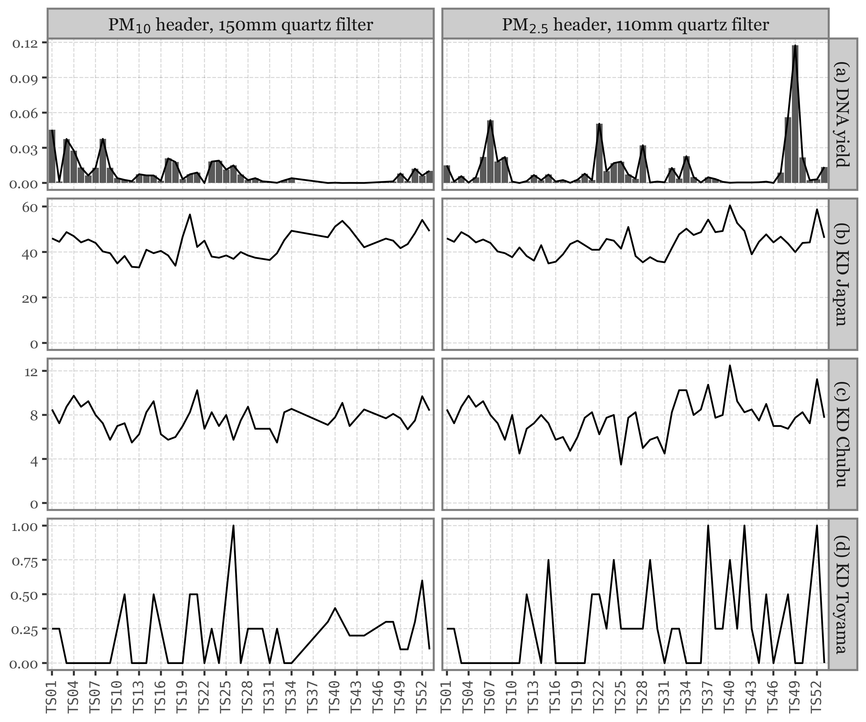
Show Code
corrs = (toyama_comp_ts
 .reset_index()
 .pivot(index='sample_id', columns='header')
 .corr(method=lambda x, y: spearmanr(x, y)[0])
 .loc['norm_dna']
 .reset_index()
 .melt([('header', '')], value_name='Spearman\'s r')
 .loc[lambda dd: dd[('header', '')] == dd['header']]
 .iloc[:6]
 .drop(columns=[('header', '')])
 .rename(columns={None: 'variable'})
 .replace({'variable': {'cases_japan': 'KD Japan',
                        'cases_chubu': 'KD Chubu',
                        'cases_toyama': 'KD Toyama'}})
 .pivot(index='variable', columns='header')
)

pvals = (toyama_comp_ts
 .reset_index()
 .pivot(index='sample_id', columns='header')
 .corr(method=lambda x, y: spearmanr(x, y)[1])
 .loc['norm_dna']
 .reset_index()
 .melt([('header', '')], value_name='p-value')
 .loc[lambda dd: dd[('header', '')] == dd['header']]
 .iloc[:6]
 .drop(columns=[('header', '')])
 .rename(columns={None: 'variable'})
 .replace({'variable': {'cases_japan': 'KD Japan',
                        'cases_chubu': 'KD Chubu',
                        'cases_toyama': 'KD Toyama'}})
 .pivot(index='variable', columns='header')
)

pd.concat([corrs, pvals], axis=1)| Spearman's r | p-value | |||
|---|---|---|---|---|
| header | PM10 | PM2.5 | PM10 | PM2.5 |
| variable | ||||
|
Loading ITables v2.1.4 from the init_notebook_mode cell...
(need help?) |
||||
In the case of Toyama, none of the DNA series for both PM2.5 and PM10 headers show any significant correlation whatsoever with their corresponding incidence of KD in Toyama, Chubu, or Japan.
Again, and given the fact that the weekly samples might be affecting the results, we will repeat the analysis but only for the daily samples:
Show Code
pacbio_toyama = (pacbio_metrics.query('sample_id.str.startswith("TS")')
 .assign(sample_id=lambda dd: 'TS' + dd.sample_id.str.split('.').str[0].str[2:].str.zfill(2))
)

toyama_comp_ts_daily = (toyama_calendar
 .query('sample_id.notna()')
 .assign(start_hour=lambda dd: np.where(dd.date == dd.start_date, dd.start_dt.dt.hour, 0))
 .query('start_hour < 12')
 .query('duration < 25')
 .groupby('sample_id')
 .apply(lambda dd: dd
        .query('date==date.max()')
        .assign(date=[pd.date_range(dd.date.min(), dd.date.max() + pd.to_timedelta(3, unit='D'))])
        ['date'])
 .reset_index()
 .explode('date')
 .merge(samples_info[['sample_id', 'header', 'volume']])
 .assign(sample_id=lambda dd: 'TS' + dd.sample_id.str.split('.').str[0].str[2:].str.zfill(2))
 .merge(kd_japan[['date', 'cases']].rename(columns={'cases': 'cases_japan'}), how='left')
 .merge(kd_chubu[['date', 'cases']].rename(columns={'cases': 'cases_chubu'}), how='left')
 .merge(kd_toyama[['date', 'cases']].rename(columns={'cases': 'cases_toyama'}), how='left')
 .merge(pacbio_toyama[['sample_id', 'header', 'dna_total']])
 .assign(norm_dna=lambda dd: dd.dna_total / dd['volume'])
 .groupby(['sample_id', 'header'])
 .agg({'cases_toyama': 'mean', 'cases_chubu': 'mean', 'cases_japan': 'mean', 'norm_dna': 'mean'})

)

(toyama_comp_ts_daily
 .reset_index()
 .melt(['sample_id', 'header'])
 .replace({'variable': {'cases_japan': '(b) KD Japan',
                        'cases_chubu': '(c) KD Chubu',
                        'cases_toyama': '(d) KD Toyama',
                         'norm_dna': '(a) DNA yield'}})
 .replace({'header': {'PM2.5': 'PM$_{2.5}$ header, 110mm quartz filter',
                      'PM10': 'PM$_{10}$ header, 150mm quartz filter'}})

 .pipe(lambda dd: p9.ggplot(dd)
       + p9.aes(x='sample_id', y='value')
       + p9.geom_col(p9.aes(alpha='variable'))
       + p9.geom_line(p9.aes(group='variable'))
       + p9.scale_alpha_manual([1, 0, 0, 0])
       + p9.scale_x_discrete(breaks=sorted(dd.sample_id.unique())[::3])
       + p9.facet_grid('variable ~ header', scales='free_y')
       + p9.guides(color=False, alpha=False)
       + p9.labs(x='', y='')
       + p9.theme(figure_size=(6, 5),
                  axis_text_x=p9.element_text(angle=90, size=7, family='monospace'),
                  axis_text_y=p9.element_text(size=7),
       )
       )
 )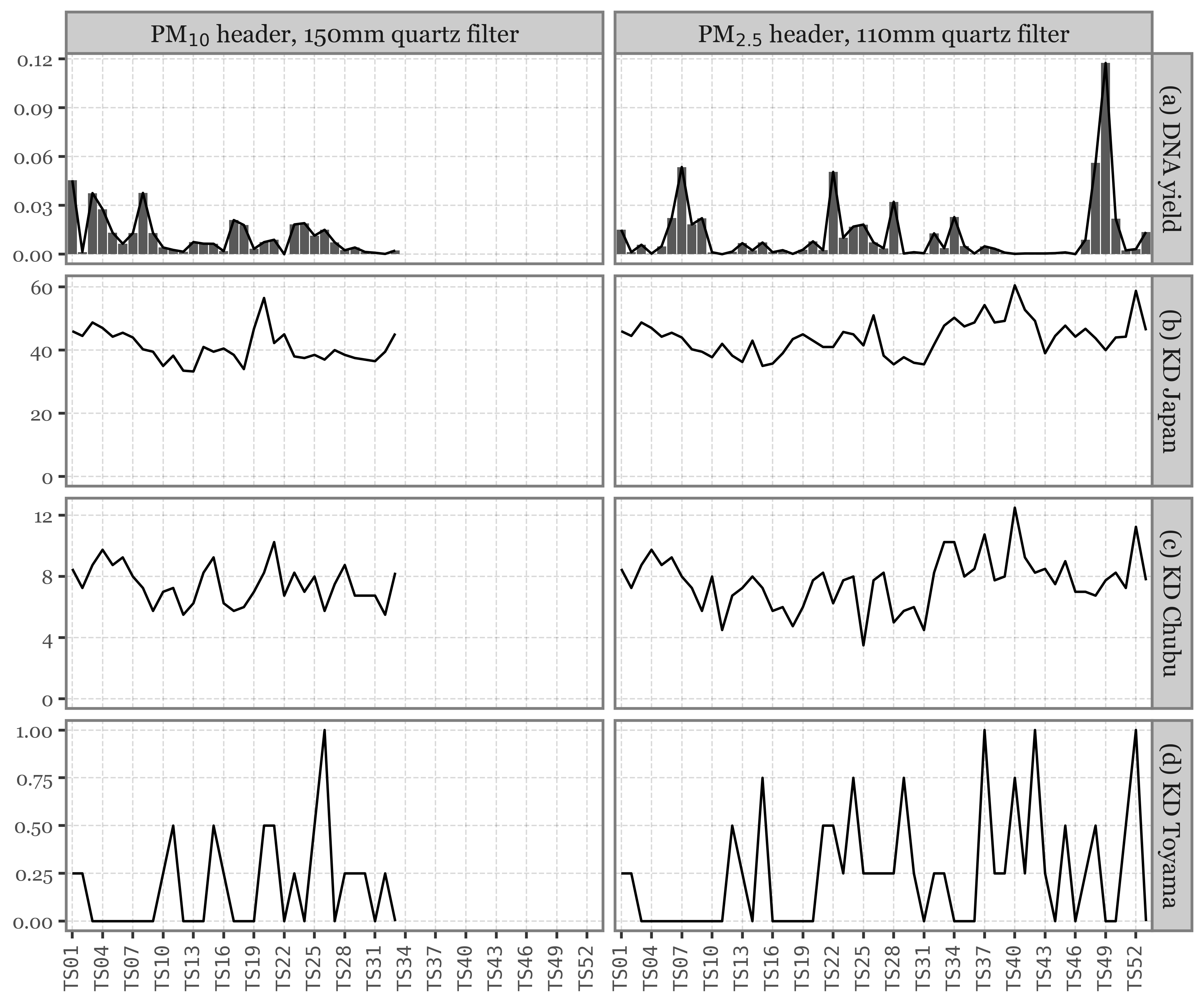
Show Code
corrs = (toyama_comp_ts_daily
 .reset_index()
 .pivot(index='sample_id', columns='header')
 .corr(method=lambda x, y: spearmanr(x, y)[0])
 .loc['norm_dna']
 .reset_index()
 .melt([('header', '')], value_name='Spearman\'s r')
 .loc[lambda dd: dd[('header', '')] == dd['header']]
 .iloc[:6]
 .drop(columns=[('header', '')])
 .rename(columns={None: 'variable'})
 .replace({'variable': {'cases_japan': 'KD Japan',
                        'cases_chubu': 'KD Chubu',
                        'cases_toyama': 'KD Toyama'}})
 .pivot(index='variable', columns='header')
)

pvals = (toyama_comp_ts_daily
 .reset_index()
 .pivot(index='sample_id', columns='header')
 .corr(method=lambda x, y: spearmanr(x, y)[1])
 .loc['norm_dna']
 .reset_index()
 .melt([('header', '')], value_name='p-value')
 .loc[lambda dd: dd[('header', '')] == dd['header']]
 .iloc[:6]
 .drop(columns=[('header', '')])
 .rename(columns={None: 'variable'})
 .replace({'variable': {'cases_japan': 'KD Japan',
                        'cases_chubu': 'KD Chubu',
                        'cases_toyama': 'KD Toyama'}})
 .pivot(index='variable', columns='header')
)

pd.concat([corrs, pvals], axis=1)| Spearman's r | p-value | |||
|---|---|---|---|---|
| header | PM10 | PM2.5 | PM10 | PM2.5 |
| variable | ||||
|
Loading ITables v2.1.4 from the init_notebook_mode cell...
(need help?) |
||||
Without the weekly samples, the associations remain the same.
Association of specific taxa with KD incidence
The association of the presence and abundance of different microbial taxa with the incidence of Kawasaki Disease is not trivial, but we will try to do our best to assess it.
Kumamoto
For starters, for Kumamoto, we have a total of 115 samples, each of them associated to a KD incidence value for the prefecture, the section, and the whole of Japan. In this 115 samples, we also have a total of 1882 fungal and bacterial genera (and I am not even taking into account the species level or the other kingdoms).
If we look at the distribution of the presence of these genera in the samples, we can see how most of them are only present in a few samples:
Show Code
(kumamoto_genera
.query('relative_abundance > 0')
.groupby('Genus', as_index=False)
.size()
.pipe(lambda dd: p9.ggplot(dd)
      + p9.geom_histogram(p9.aes('size', alpha='size >= 20'), binwidth=2, color='black', size=.2)
      + p9.scale_x_continuous(expand=(0.0075, 0.0075))
      + p9.scale_y_continuous(expand=(.0075, 0, .01, 0))
      + p9.guides(alpha=False)
      + p9.annotate('vline', xintercept=19, color='red', size=.5, linetype='dashed')
      + p9.annotate('text', x=22, y=500, label='Selected (at least present in 20 samples)',
                     size=7, ha='left')
      + p9.labs(x='Presence in $n$ samples', y='Number of genera',
                title='Distribution of genera by presence in Kumamoto samples')
      + p9.theme(figure_size=(3.5, 2),
                 axis_text=p9.element_text(size=7),
                 axis_title=p9.element_text(size=8),
                 plot_title=p9.element_text(size=8.5)
                 )

)
)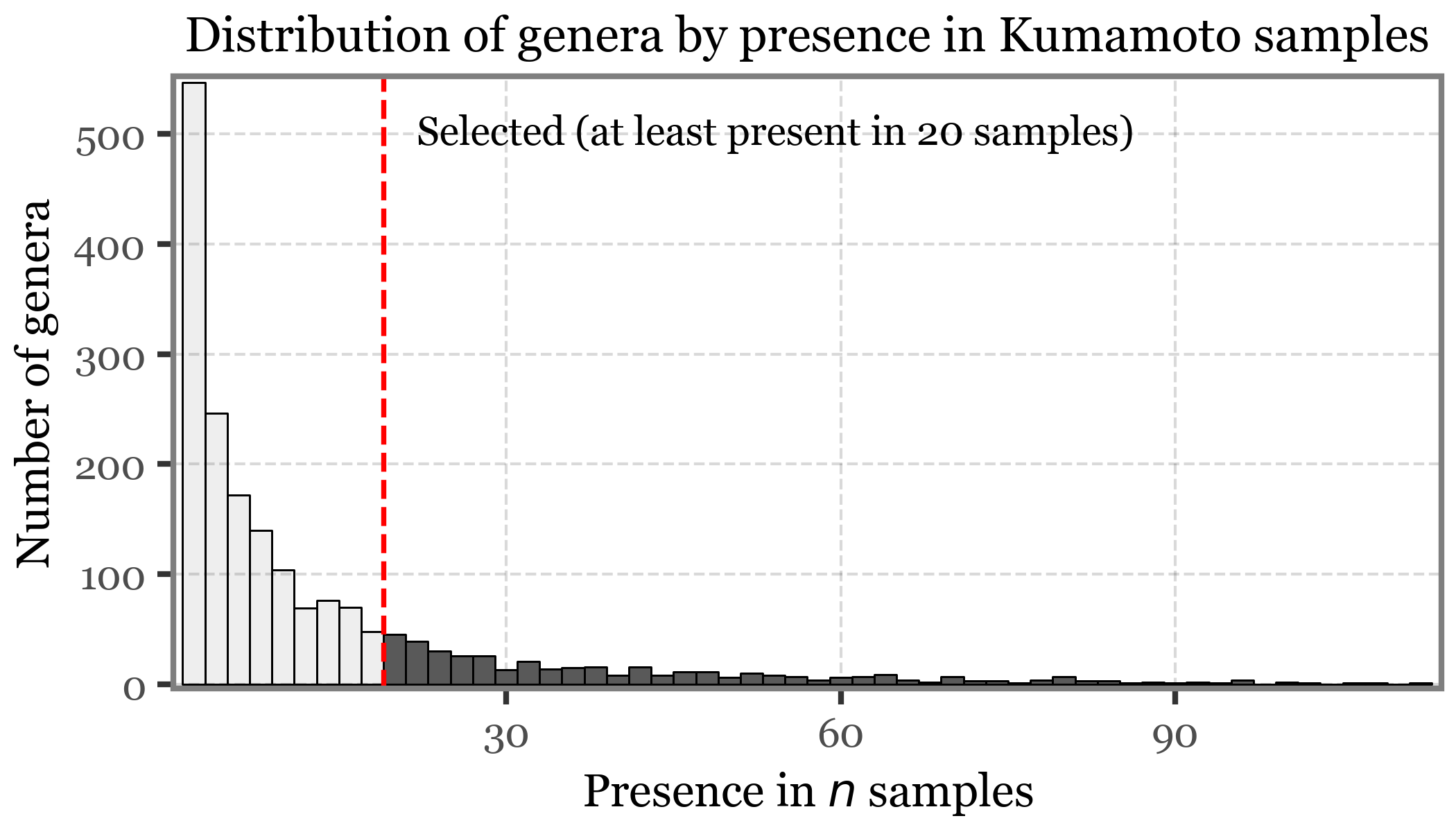
Given this, to reduce the number of tests and variables to consider, we will filter out all the genera that are not present in at least 20 different samples. This leaves us with a total of 387 fungal and bacterial genera to consider.
A smarter approach would be now to cluster the genera by their relative abundance across samples and then use the clusters as variables to correlate with the KD incidence. However, at this point, we will just use the relative abundance of each genus in each sample as a variable to correlate with the KD incidence.
Data preparation for genera matrix and kd comparison
missing_samples = (kumamoto_genera
 .groupby(['sample_id', 'Kingdom'], as_index=False)
 .relative_abundance.sum()
 .query('relative_abundance == 0')
 ['sample_id']
)

genera_over_20_samples = (kumamoto_genera
.query('relative_abundance > 0')
.groupby('Genus', as_index=False)
.size()
.query('size > 20')
['Genus']
)

kumamoto_genera_matrix = (kumamoto_genera
 .query('Genus in @genera_over_20_samples')
 .query('not sample_id in @missing_samples')
 .pivot(index='sample_id', columns='Genus', values='relative_abundance')
 )

genus_kyushu_comp = pd.concat([kumamoto_genera_matrix
 .corrwith(kumamoto_comp_ts['cases_kyushu'],
            method=lambda x, y: spearmanr(x, y)[0])
 .rename('r'),
    kumamoto_genera_matrix.corrwith(kumamoto_comp_ts['cases_kyushu'],
                                     method=lambda x, y: spearmanr(x, y)[1])
 .rename('p-value')
], axis=1).assign(comp='KD Kyushu')

genus_japan_comp = pd.concat([kumamoto_genera_matrix
    .corrwith(kumamoto_comp_ts['cases_japan'],
                method=lambda x, y: spearmanr(x, y)[0])
    .rename('r'),
        kumamoto_genera_matrix.corrwith(kumamoto_comp_ts['cases_japan'],
                                        method=lambda x, y: spearmanr(x, y)[1])
    .rename('p-value')
    ], axis=1).assign(comp='KD Japan')

genus_kumamoto_comp = pd.concat([kumamoto_genera_matrix
    .corrwith(kumamoto_comp_ts['cases_kumamoto'],
                method=lambda x, y: spearmanr(x, y)[0])
    .rename('r'),
        kumamoto_genera_matrix.corrwith(kumamoto_comp_ts['cases_kumamoto'],
                                        method=lambda x, y: spearmanr(x, y)[1])
    .rename('p-value')
    ], axis=1).assign(comp='KD Kumamoto')

k_g_map = kumamoto_genera[['Kingdom', 'Genus']].drop_duplicates()

selected_genus = pd.concat([
    genus_kyushu_comp.query('`p-value` < .05').reset_index(),
    genus_kumamoto_comp.query('`p-value` < .05').reset_index(),
    genus_japan_comp.query('`p-value` < .05').reset_index()
])
If we select only those genera with significant correlation with any of the KD incidence values in either direction, we get the following results:
Show Code
(selected_genus
 .merge(k_g_map, on='Genus')
 .assign(comp=lambda dd: pd.Categorical(dd.comp, categories=['KD Kumamoto', 'KD Kyushu', 'KD Japan']))
 .pipe(lambda dd: p9.ggplot(dd)
       + p9.aes('reorder(Genus, r)', 'r')
       + p9.geom_col(p9.aes(fill='r'))
       + p9.scale_fill_continuous('RdBu', limits=(-.3, .3))
       + p9.coord_flip()
       + p9.guides(fill=False)
       + p9.labs(x='', y="Spearman's r",)
       + p9.facet_wrap('~comp', scales='free_y')
       + p9.theme(figure_size=(8, 6))
       )
)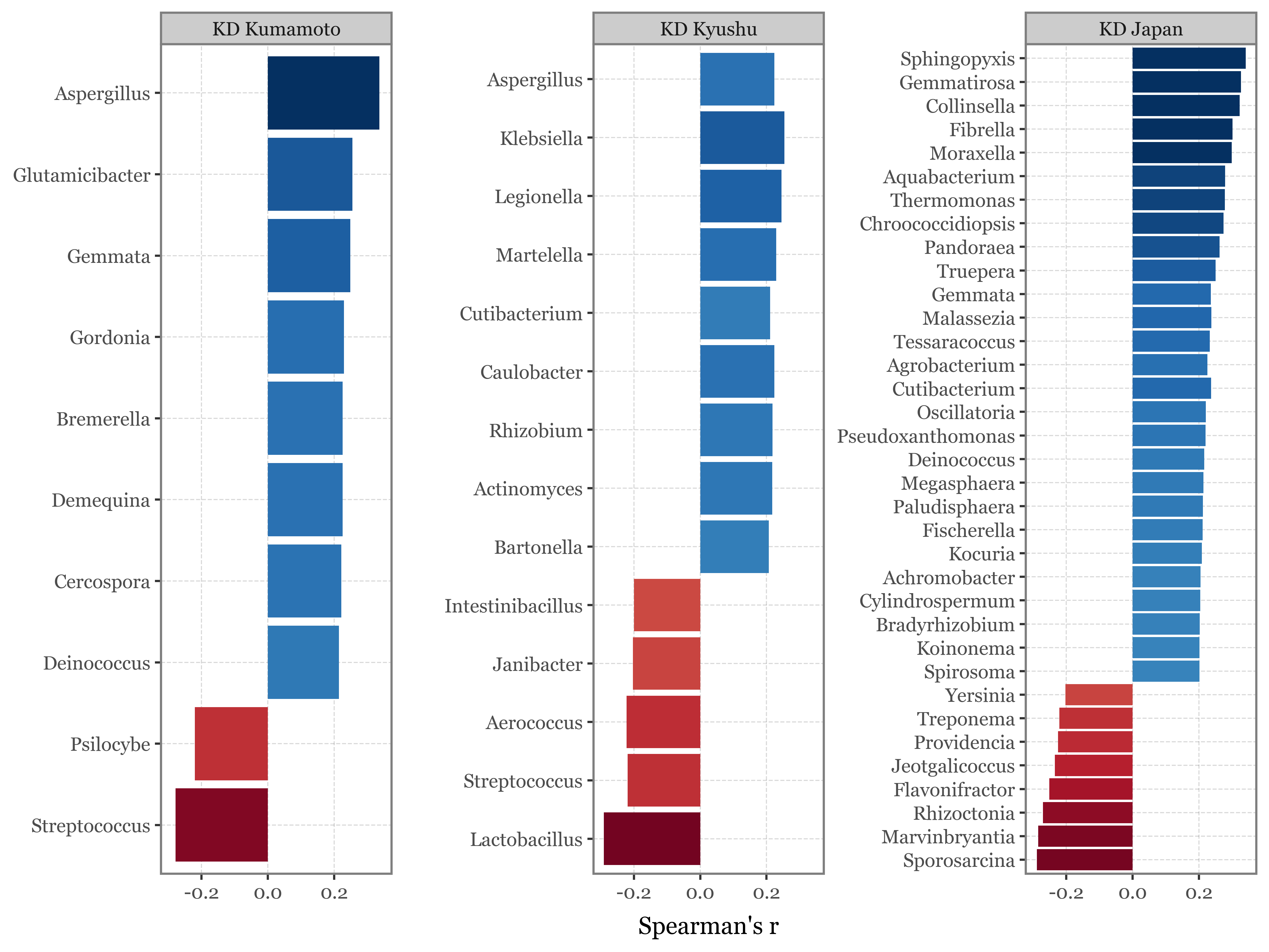
The full table is the following:
Show Code
show(selected_genus.style.format({'r': '{:.3f}', 'p-value': '{:.3f}'}).hide(axis=0),
        buttons=['csv'], pageLength=60,
)| Genus | r | p-value | comp |
|---|---|---|---|
| Actinomyces | 0.218 | 0.031 | KD Kyushu |
| Aerococcus | -0.222 | 0.028 | KD Kyushu |
| Aspergillus | 0.224 | 0.027 | KD Kyushu |
| Bartonella | 0.207 | 0.041 | KD Kyushu |
| Caulobacter | 0.224 | 0.027 | KD Kyushu |
| Cutibacterium | 0.211 | 0.037 | KD Kyushu |
| Intestinibacillus | -0.200 | 0.048 | KD Kyushu |
| Janibacter | -0.203 | 0.045 | KD Kyushu |
| Klebsiella | 0.254 | 0.012 | KD Kyushu |
| Lactobacillus | -0.291 | 0.004 | KD Kyushu |
| Legionella | 0.246 | 0.015 | KD Kyushu |
| Martelella | 0.229 | 0.023 | KD Kyushu |
| Rhizobium | 0.218 | 0.031 | KD Kyushu |
| Streptococcus | -0.219 | 0.030 | KD Kyushu |
| Aspergillus | 0.337 | 0.001 | KD Kumamoto |
| Bremerella | 0.226 | 0.025 | KD Kumamoto |
| Cercospora | 0.222 | 0.028 | KD Kumamoto |
| Deinococcus | 0.215 | 0.034 | KD Kumamoto |
| Demequina | 0.225 | 0.026 | KD Kumamoto |
| Gemmata | 0.249 | 0.013 | KD Kumamoto |
| Glutamicibacter | 0.256 | 0.011 | KD Kumamoto |
| Gordonia | 0.230 | 0.023 | KD Kumamoto |
| Psilocybe | -0.221 | 0.029 | KD Kumamoto |
| Streptococcus | -0.278 | 0.006 | KD Kumamoto |
| Achromobacter | 0.205 | 0.043 | KD Japan |
| Agrobacterium | 0.226 | 0.025 | KD Japan |
| Aquabacterium | 0.279 | 0.005 | KD Japan |
| Bradyrhizobium | 0.202 | 0.046 | KD Japan |
| Chroococcidiopsis | 0.274 | 0.006 | KD Japan |
| Collinsella | 0.323 | 0.001 | KD Japan |
| Cutibacterium | 0.237 | 0.019 | KD Japan |
| Cylindrospermum | 0.204 | 0.044 | KD Japan |
| Deinococcus | 0.216 | 0.032 | KD Japan |
| Fibrella | 0.301 | 0.003 | KD Japan |
| Fischerella | 0.211 | 0.037 | KD Japan |
| Flavonifractor | -0.251 | 0.013 | KD Japan |
| Gemmata | 0.236 | 0.019 | KD Japan |
| Gemmatirosa | 0.327 | 0.001 | KD Japan |
| Jeotgalicoccus | -0.234 | 0.020 | KD Japan |
| Kocuria | 0.209 | 0.039 | KD Japan |
| Koinonema | 0.202 | 0.046 | KD Japan |
| Malassezia | 0.238 | 0.018 | KD Japan |
| Marvinbryantia | -0.285 | 0.005 | KD Japan |
| Megasphaera | 0.214 | 0.034 | KD Japan |
| Moraxella | 0.299 | 0.003 | KD Japan |
| Oscillatoria | 0.221 | 0.029 | KD Japan |
| Paludisphaera | 0.212 | 0.036 | KD Japan |
| Pandoraea | 0.263 | 0.009 | KD Japan |
| Providencia | -0.225 | 0.026 | KD Japan |
| Pseudoxanthomonas | 0.220 | 0.030 | KD Japan |
| Rhizoctonia | -0.270 | 0.007 | KD Japan |
| Sphingopyxis | 0.342 | 0.001 | KD Japan |
| Spirosoma | 0.202 | 0.047 | KD Japan |
| Sporosarcina | -0.289 | 0.004 | KD Japan |
| Tessaracoccus | 0.233 | 0.021 | KD Japan |
| Thermomonas | 0.279 | 0.005 | KD Japan |
| Treponema | -0.221 | 0.029 | KD Japan |
| Truepera | 0.250 | 0.013 | KD Japan |
| Yersinia | -0.203 | 0.045 | KD Japan |
Toyama
For the case of Toyama, given the two different headers, we will split the analysis by header type.
The number of samples for each header is then the following:
Show Code
(toyama_genera
.query('relative_abundance > 0')
.groupby(['header'])
.sample_id.nunique()
.rename('Number of samples with data')
)| Number of samples with data | |
|---|---|
| header | |
|
Loading ITables v2.1.4 from the init_notebook_mode cell...
(need help?) |
To account for the lower number of samples with respect to the Kumamoto case, we will lower the filter to include all those genera that are present in at least 10 samples. The distribution of the presence of these genera and the filtering looks like this then:
Show Code
(toyama_genera
.query('relative_abundance > 0')
.groupby(['header', 'Genus'], as_index=False)
.size()
.pipe(lambda dd: p9.ggplot(dd)
      + p9.geom_histogram(p9.aes('size', alpha='size >= 10'), binwidth=2, color='black', size=.2)
      + p9.scale_x_continuous(expand=(0.0075, 0.0075))
      + p9.scale_y_continuous(expand=(.0075, 0, .01, 0))
      + p9.guides(alpha=False)
      + p9.facet_wrap('header', ncol=1)
      + p9.annotate('vline', xintercept=9, color='red', size=.5, linetype='dashed')
      + p9.annotate('text', x=12, y=500, label='Selected (at least present in 10 samples)',
                     size=7, ha='left')
      + p9.labs(x='Presence in $n$ samples', y='Number of genera',
                title='Distribution of genera by presence in Toyama samples')
      + p9.theme(figure_size=(3.5, 4),
                 axis_text=p9.element_text(size=7),
                 axis_title=p9.element_text(size=8),
                 plot_title=p9.element_text(size=8.5)
                 )

)
)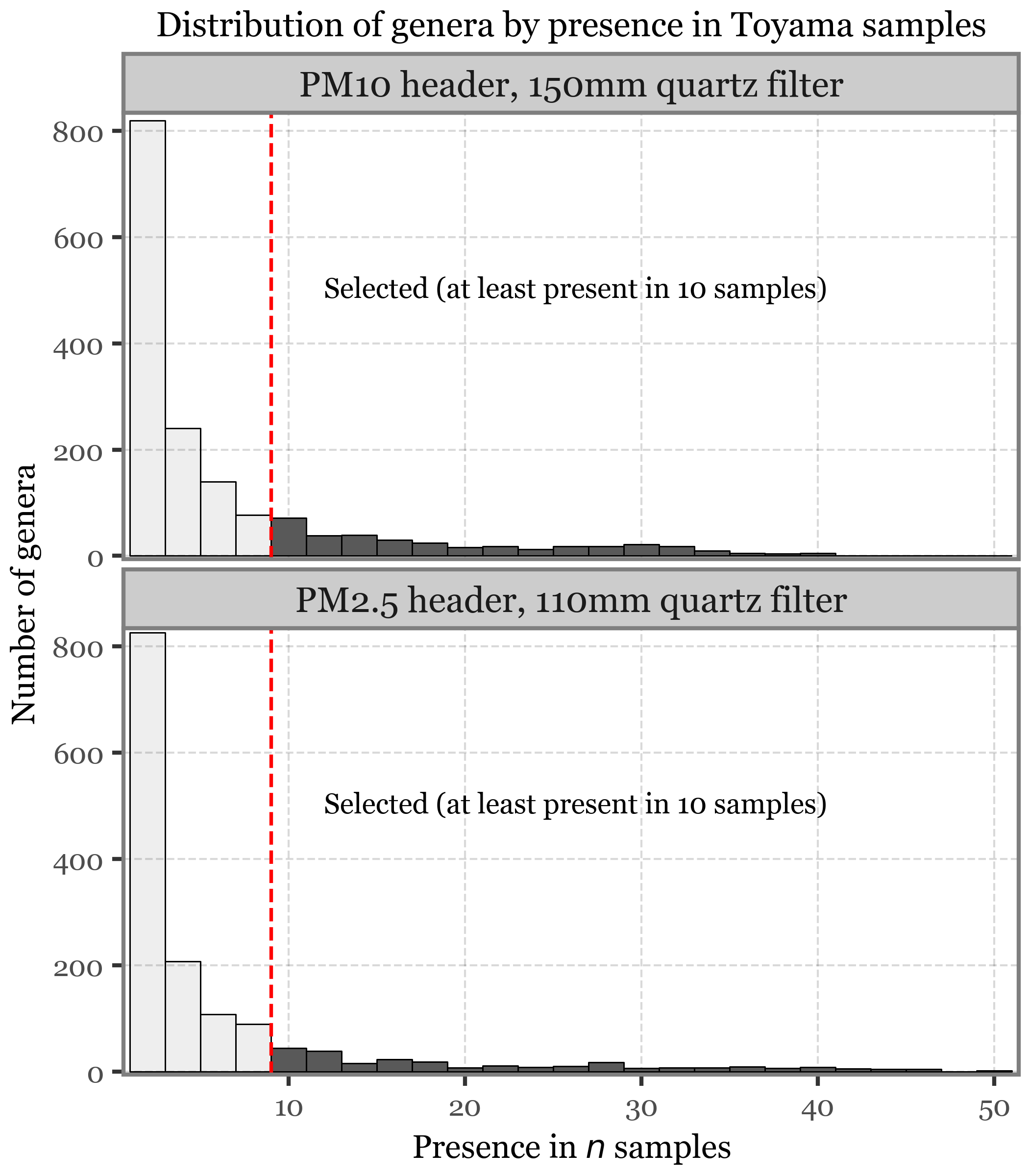
Data preparation for genera matrix and KD comparison
missing_samples_pm25 = (toyama_genera
 .query('header=="PM2.5 header, 110mm quartz filter"')
 .groupby(['sample_id', 'Kingdom'], as_index=False)
 .relative_abundance.sum()
 .query('relative_abundance == 0')
 ['sample_id']
)

missing_samples_pm10 = (toyama_genera
    .query('header=="PM10 header, 150mm quartz filter"')
    .groupby(['sample_id', 'Kingdom'], as_index=False)
    .relative_abundance.sum()
    .query('relative_abundance == 0')
    ['sample_id']
)

genera_over_10_samples_pm25 = (toyama_genera
    .query('header=="PM2.5 header, 110mm quartz filter"')
    .query('relative_abundance > 0')
    .groupby('Genus', as_index=False)
    .size()
    .query('size >= 10')
    ['Genus']
)

genera_over_10_samples_pm10 = (toyama_genera
    .query('header=="PM10 header, 150mm quartz filter"')
    .query('relative_abundance > 0')
    .groupby('Genus', as_index=False)
    .size()
    .query('size >= 10')
    ['Genus']
)

toyama_genera_matrix_pm25 = (toyama_genera
 .query('header=="PM2.5 header, 110mm quartz filter"')
 .query('Genus in @genera_over_20_samples')
 .query('not sample_id in @missing_samples')
 .pivot(index='sample_id', columns='Genus', values='relative_abundance')
 )


toyama_genera_matrix_pm10 = (toyama_genera
    .query('header=="PM10 header, 150mm quartz filter"')
    .query('Genus in @genera_over_20_samples')
    .query('not sample_id in @missing_samples')
    .pivot(index='sample_id', columns='Genus', values='relative_abundance')
    )


genus_chubu_comp_pm25 = pd.concat([toyama_genera_matrix_pm25
    .corrwith(toyama_comp_ts['cases_chubu'],
                method=lambda x, y: spearmanr(x, y)[0])
    .rename('r'),
        toyama_genera_matrix_pm25.corrwith(toyama_comp_ts['cases_chubu'],
                                        method=lambda x, y: spearmanr(x, y)[1])
    .rename('p-value')
    ], axis=1).assign(comp='KD Chubu')

genus_japan_comp_pm25 = pd.concat([toyama_genera_matrix_pm25
    .corrwith(toyama_comp_ts['cases_japan'],
                method=lambda x, y: spearmanr(x, y)[0])
    .rename('r'),
        toyama_genera_matrix_pm25.corrwith(toyama_comp_ts['cases_japan'],
                                        method=lambda x, y: spearmanr(x, y)[1])
    .rename('p-value')
    ], axis=1).assign(comp='KD Japan')

genus_toyama_comp_pm25 = pd.concat([toyama_genera_matrix_pm25
    .corrwith(toyama_comp_ts['cases_toyama'],
                method=lambda x, y: spearmanr(x, y)[0])
    .rename('r'),
        toyama_genera_matrix_pm25.corrwith(toyama_comp_ts['cases_toyama'],
                                        method=lambda x, y: spearmanr(x, y)[1])
    .rename('p-value')
    ], axis=1).assign(comp='KD Toyama')

genus_chubu_comp_pm10 = pd.concat([toyama_genera_matrix_pm10
    .corrwith(toyama_comp_ts['cases_chubu'],
                method=lambda x, y: spearmanr(x, y)[0])
    .rename('r'),
        toyama_genera_matrix_pm10.corrwith(toyama_comp_ts['cases_chubu'],
                                        method=lambda x, y: spearmanr(x, y)[1])
    .rename('p-value')
    ], axis=1).assign(comp='KD Chubu')

genus_japan_comp_pm10 = pd.concat([toyama_genera_matrix_pm10
    .corrwith(toyama_comp_ts['cases_japan'],
                method=lambda x, y: spearmanr(x, y)[0])
    .rename('r'),
        toyama_genera_matrix_pm10.corrwith(toyama_comp_ts['cases_japan'],
                                        method=lambda x, y: spearmanr(x, y)[1])
    .rename('p-value')
    ], axis=1).assign(comp='KD Japan')

genus_toyama_comp_pm10 = pd.concat([toyama_genera_matrix_pm10
    .corrwith(toyama_comp_ts['cases_toyama'],
                method=lambda x, y: spearmanr(x, y)[0])
    .rename('r'),
        toyama_genera_matrix_pm10.corrwith(toyama_comp_ts['cases_toyama'],
                                        method=lambda x, y: spearmanr(x, y)[1])
    .rename('p-value')
    ], axis=1).assign(comp='KD Toyama')

k_g_map = toyama_genera[['Kingdom', 'Genus']].drop_duplicates()

selected_genus_pm25 = pd.concat([
    genus_chubu_comp_pm25.query('`p-value` < .05').reset_index(),
    genus_toyama_comp_pm25.query('`p-value` < .05').reset_index(),
    genus_japan_comp_pm25.query('`p-value` < .05').reset_index()
])

selected_genus_pm10 = pd.concat([
    genus_chubu_comp_pm10.query('`p-value` < .05').reset_index(),
    genus_toyama_comp_pm10.query('`p-value` < .05').reset_index(),
    genus_japan_comp_pm10.query('`p-value` < .05').reset_index()
])
Again, if we only select the significant correlations (at a fairly relaxed \(\alpha=0.05\) non-adjusted), we get the following results:
Show Code
(selected_genus_pm10
 .merge(k_g_map, on='Genus')
 .assign(comp=lambda dd: pd.Categorical(dd.comp, categories=['KD Toyama', 'KD Chubu', 'KD Japan']))
 .pipe(lambda dd: p9.ggplot(dd)
       + p9.aes('reorder(Genus, r)', 'r')
       + p9.geom_col(p9.aes(fill='r'))
       + p9.scale_fill_continuous('RdBu', limits=(-.5, .5))
       + p9.coord_flip()
       + p9.guides(fill=False)
       + p9.labs(x='', y="Spearman's r",
                 title='Correlation of bacterial and fungal genera with KD cases (PM$_{10}$ header)')
       + p9.facet_wrap('~comp', scales='free_y')
       + p9.theme(figure_size=(9, 10))
       )
)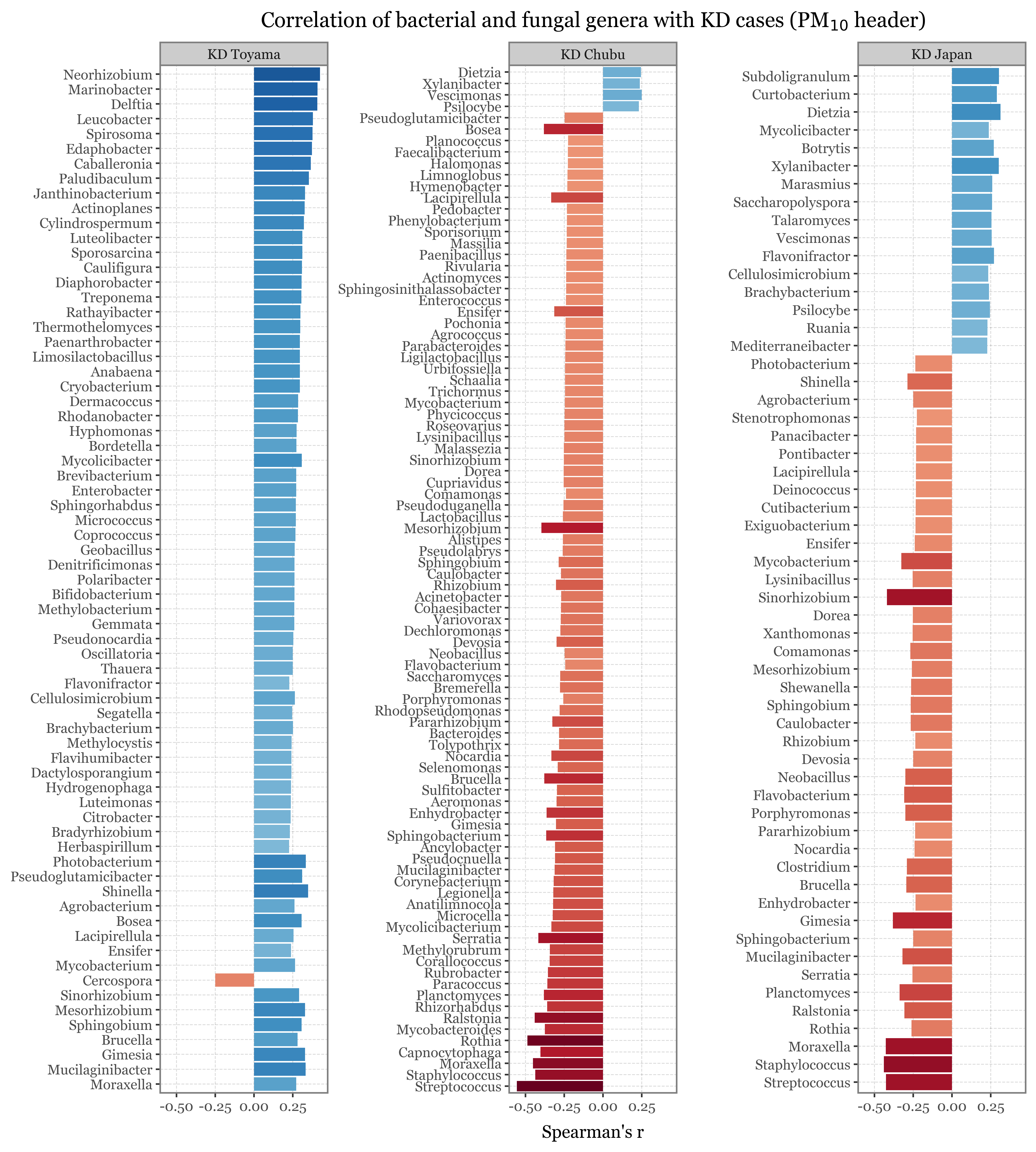
Show Code
(selected_genus_pm25
 .merge(k_g_map, on='Genus')
 .assign(comp=lambda dd: pd.Categorical(dd.comp, categories=['KD Toyama', 'KD Chubu', 'KD Japan']))
 .pipe(lambda dd: p9.ggplot(dd)
       + p9.aes('reorder(Genus, r)', 'r')
       + p9.geom_col(p9.aes(fill='r'))
       + p9.scale_fill_continuous('RdBu', limits=(-.5, .5))
       + p9.coord_flip()
       + p9.guides(fill=False)
       + p9.labs(x='', y="Spearman's r",
                 title='Correlation of bacterial and fungal genera with KD cases (PM$_{2.5}$ header)')
       + p9.facet_wrap('~comp', scales='free_y')
       + p9.theme(figure_size=(9, 10))
       )
)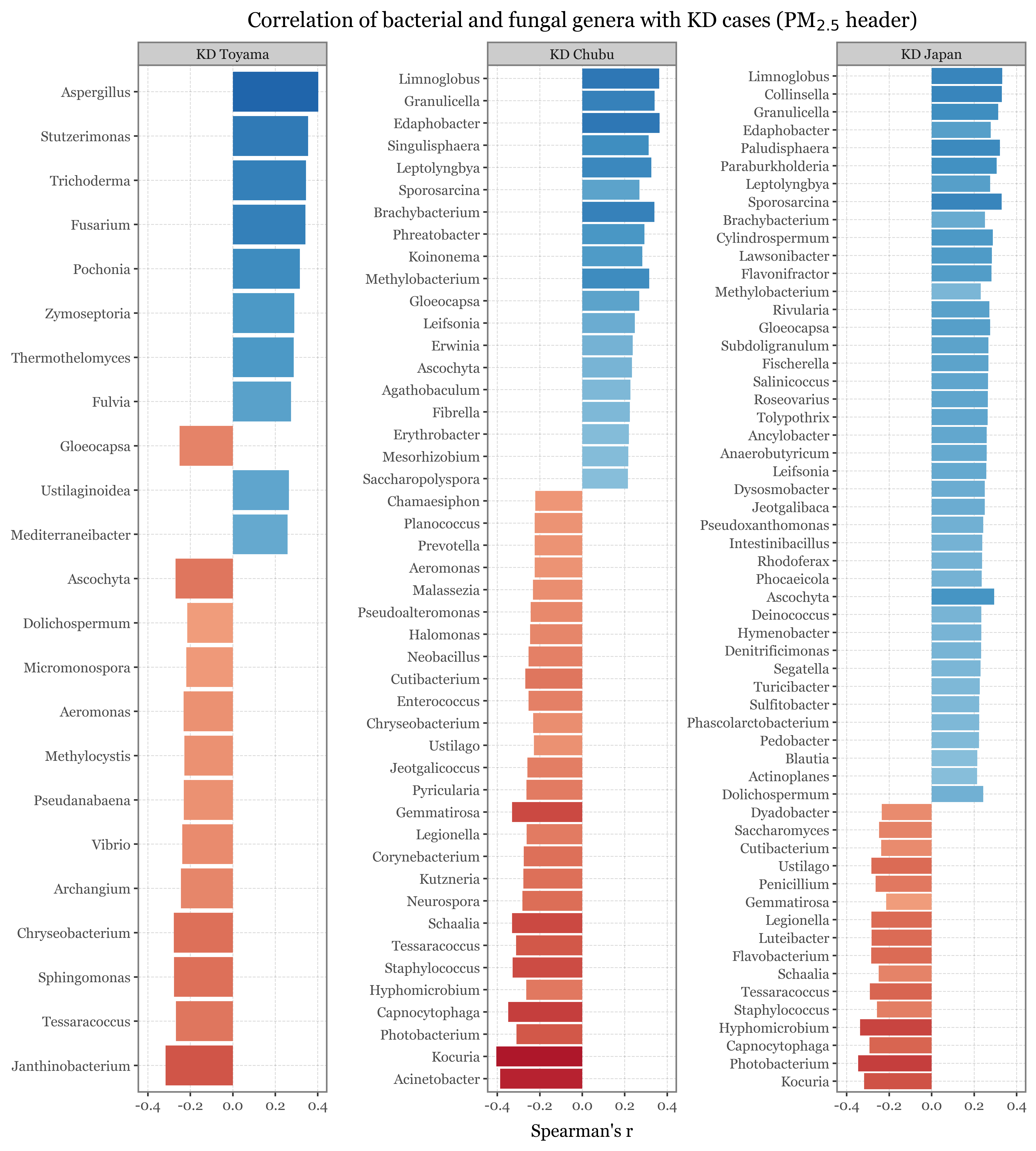
These are all fairly weak correlation, or at least the expected ones taking into account the sheer number of tests we are performing, with the direction of the correlation going either way.
Better methods can be applied, but I am leaving this here for now until we have some better feedback on several of the issues raised up to know with respect to the data and the arbitrary choices made on the way.
References
Gusareva, Elena S, Enzo Acerbi, Kenny JX Lau, Irvan Luhung, Balakrishnan NV Premkrishnan, Sandra Kolundžija, Rikky W Purbojati, et al. 2019. “Microbial Communities in the Tropical Air Ecosystem Follow a Precise Diel Cycle.” Proceedings of the National Academy of Sciences 116 (46): 23299–308.
Rodó, Xavier, Albert Navarro-Gallinad, Tomoko Kojima, Josep-Anton Morguı́, Silvia Borràs, and Alejandro Fontal. 2023. “Sub-Weekly Signatures Relate Ultrafine Aerosols Enriched in Metals from Intensive Farming and Urban Pollution to Kawasaki Disease.” Environmental Research Letters 18 (7): 074011.