Assembled contigs vs long HiFi reads for taxonomic classification

Testing out the new Pacbio metagenomics workflow for air samples

Authors

Affiliations

Alejandro Fontal

Climate & Health Program, ISGlobal

Daniel Ekhlas

AIRLAB, Climate & Health Program, ISGlobal

Xavier Rodó

Climate & Health Program, ISGlobal

Catalonia Institute for Advanced Studies

Published

December 15, 2025

Preamble

In this section we will load the necessary libraries and set the global parameters for the notebook. It’s irrelevant for the narrative of the analysis but essential for the reproducibility of the results. Since in this case we are using both Python and R, we have a bit of a more complex setup than usual. This includes using the rpy2 package to run R code within the Python environment, as well as ensuring that data is properly passed between the two languages.

Show code imports and presets

Code imports

import os
import warnings

warnings.filterwarnings("ignore", category=UserWarning, module="rpy2")

# Clean environment variables that cause issues with R
# Remove bash functions that R can't parse properly
env_vars_to_remove = ["BASH_FUNC_ml%%", "BASH_FUNC_module%%", "BASH_FUNC_which%%"]

for var in env_vars_to_remove:
    if var in os.environ:
        del os.environ[var]

# only if the OS is macOS and R_HOME is not set (otherwise fails...)
if os.name == "posix" and os.uname().sysname == "Darwin":
    os.environ["R_HOME"] = "/Library/Frameworks/R.framework/Resources"
%load_ext rpy2.ipython

%%R

# Load the packages
library(dplyr)
library(vegan)
library(ggplot2)
library(phyloseq)
library(magrittr)


Attaching package: ‘dplyr’

The following objects are masked from ‘package:stats’:

    filter, lag

The following objects are masked from ‘package:base’:

    intersect, setdiff, setequal, union

Loading required package: permute
This is vegan 2.7-2

import re
import numpy as np
import pandas as pd
import polars as pl
import plotnine as p9
from glob import glob
from Bio import Entrez
from pathlib import Path
from ete3 import NCBITaxa
from collections import defaultdict
from skbio.stats.ordination import pcoa
from skbio.diversity import beta_diversity
from mizani.formatters import percent_format
from scipy.spatial.distance import braycurtis

Presets

# Matplotlib settings
import matplotlib.pyplot as plt
from matplotlib_inline.backend_inline import set_matplotlib_formats

plt.rcParams["font.family"] = "IBM Plex Sans"
plt.rcParams["svg.fonttype"] = "none"
set_matplotlib_formats("retina")
plt.rcParams["figure.dpi"] = 300

# Plotnine settings (for figures)
p9.options.set_option("base_family", "IBM Plex Sans")

p9.theme_set(
    p9.theme_classic()
    + p9.theme(
        panel_grid=p9.element_blank(),
        legend_background=p9.element_blank(),
        panel_grid_major=p9.element_line(
            size=0.5, linetype="dashed", alpha=0.15, color="black"
        ),
        plot_title=p9.element_text(ha="center"),
        dpi=300,
    )
)

Entrez.email = "alejandro.fontal@isglobal.org"

Introduction

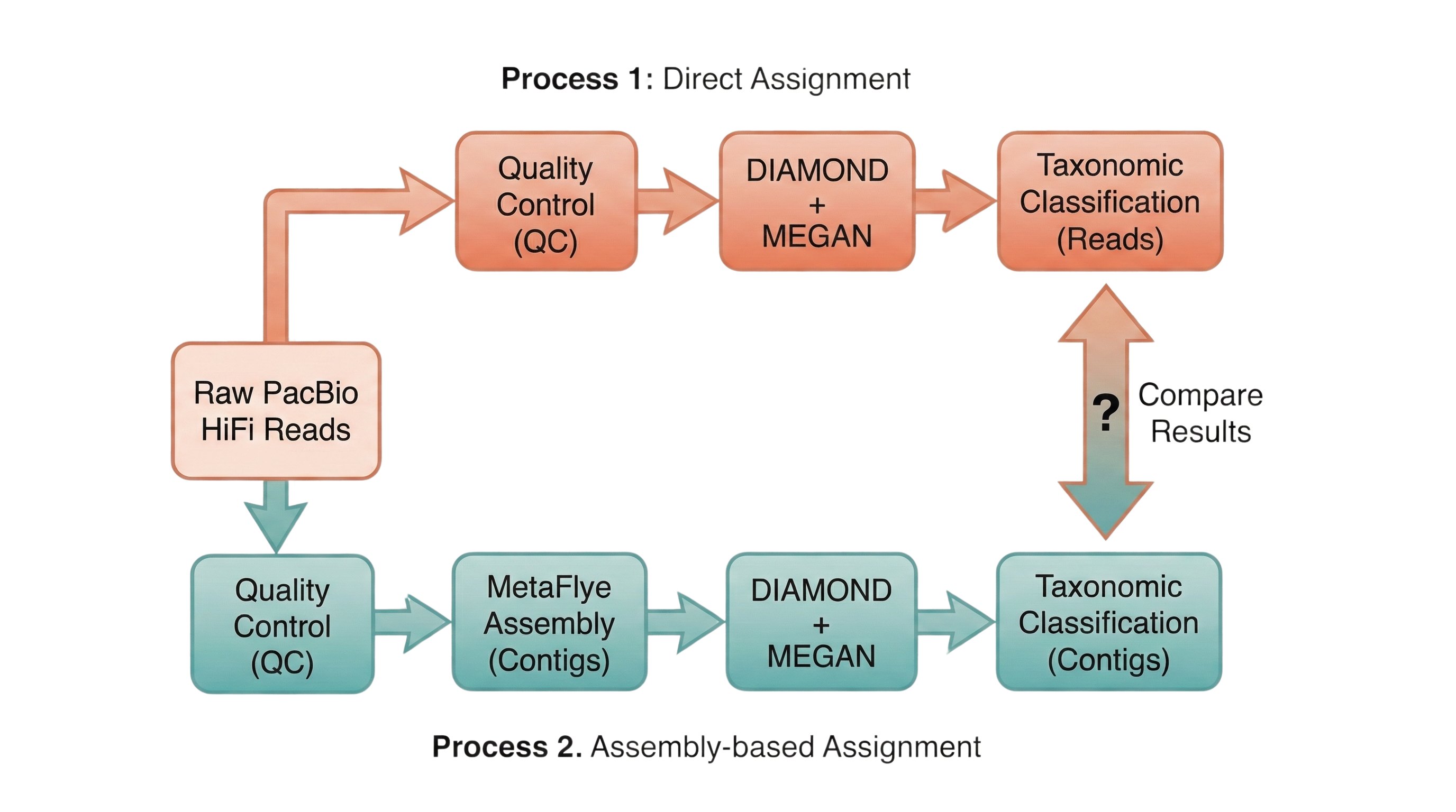
In this notebook we will try to compare the taxonomic composition of Kumamoto samples which were processed in two different ways:

Directly assigned using DIAMOND + MEGAN using the raw PacBio reads.
Assigned using DIAMOND + MEGAN using the assembled contigs from the same PacBio reads.

Our expectation is not that assemblies and long reads will give identical communities, but that they should agree on the dominant structure. Assemblies may collapse highly similar fragments into longer contigs, which can help DIAMOND+MEGAN anchor hits more confidently but may also lose very low abundance or fragmented taxa. Direct classification of long reads, on the other hand, keeps every fragment but is both noisier and much more expensive computationally. The question for these air samples (where input DNA is ultra-low and heavily amplified) is whether assemblies change the ecological picture in a meaningful way or mainly reshuffle rare taxa and strain-level detail.

The process is more expensive using direct assignment, as the number of reads is much higher and the DIAMOND + MEGAN pipeline is more resource-intensive. This has caused several crashes while trying to run the pipeline on the raw reads in ISGlobal’s HPC, so we need to see if we gain enough information to justify the extra cost.

Loading Data

For convenience, we already stored the matched samples in tsv files in the data/comparisons directory.

Let’s load them while tagging the samples with the sample name and source:

tax_dfs = []
for file in glob("../data/comparisons/assembled/*.tsv"):
    sample_name = file.split("/")[-1].split("_")[0]
    tax_dfs.append(
        pd.read_csv(file, sep="\t").assign(sample_id=sample_name).assign(kind="contigs")
    )

for file in glob("../data/comparisons/unassembled/*.tsv"):
    sample_name = file.split("/")[-1].split("_")[0]
    tax_dfs.append(
        pd.read_csv(file, sep="\t").assign(sample_id=sample_name).assign(kind="reads")
    )

tax_dfs = pd.concat(tax_dfs)[["sample_id", "kind", "taxid", "count"]]

comparable_samples = (
    tax_dfs.groupby("sample_id").kind.nunique().loc[lambda x: x == 2].index.values
)
tax_dfs = tax_dfs.query("sample_id in @comparable_samples")

Alpha-diversity comparison

For starters, we will define a small helper function to compute the alpha diversity metrics used in this analysis. Although there are packages that implement these indices, they are straightforward to calculate, and defining them here keeps the workflow explicit and transparent.

These metrics are:

Richness: counts how many taxa are present, capturing diversity in terms of number of taxa only, without considering their abundances.
Shannon diversity index: combines richness and evenness, giving more weight to rare taxa than dominance-focused indices.
Simpson diversity index: emphasizes the contribution of common taxa, providing a measure of how dominated a community is by abundant taxa.
Berger-Parker dominance: focuses on the single most abundant taxon, quantifying the degree to which one taxon dominates the community compared with the others.

def compute_alpha(group):
    counts = group["count"]
    total = counts.sum()
    p = counts / total
    # Shannon entropy
    shannon = -np.sum(p * np.log(p + 1e-9))
    # Simpson
    simpson = 1 - np.sum(p**2)
    # Berger-Parker
    berger_parker = p.max()
    # Richness
    richness = (counts > 0).sum()

    return pd.Series(
        {
            "richness": richness,
            "shannon": shannon,
            "simpson": simpson,
            "berger_parker": berger_parker,
        }
    )

If we now apply those metrics to each of the 21 samples with both methodologies, we get the following output:

Show Code

alpha_long = (
    tax_dfs.groupby(["sample_id", "kind"])
    .apply(compute_alpha, include_groups=False)
    .reset_index()
)

metric_map = {
    "richness": "Richness (unique taxa)",
    "shannon": "Shannon's diversity",
    "simpson": "Simpson's diversity",
    "berger_parker": "Berger-Parker dominance",
}
kind_map = {"reads": "HiFi reads only", "contigs": "Assembled contigs"}

sorted_samples = alpha_long.query('kind == "reads"').sort_values("richness").sample_id

alpha_long_melted = (
    alpha_long.melt(
        id_vars=["sample_id", "kind"], var_name="metric_name", value_name="value"
    )
    .assign(metric_name=lambda dd: dd.metric_name.map(metric_map))
    .assign(kind_label=lambda dd: dd.kind.map(kind_map))
    .assign(
        metric_name=lambda dd: pd.Categorical(
            dd.metric_name, categories=metric_map.values()
        )
    )
    .assign(
        sample_id=lambda dd: pd.Categorical(dd.sample_id, categories=sorted_samples)
    )
)


(
    p9.ggplot(alpha_long_melted, p9.aes(x="sample_id", y="value", fill="kind_label"))
    + p9.geom_col(position="dodge")
    + p9.coord_flip()
    + p9.facet_wrap("~metric_name", scales="free_x", ncol=4)
    + p9.scale_y_continuous(expand=(0, 0))
    + p9.labs(x="", y="", fill="")
    + p9.theme(
        legend_position="top",
        figure_size=(7, 5),
        panel_spacing_x=0.025,
    )
)

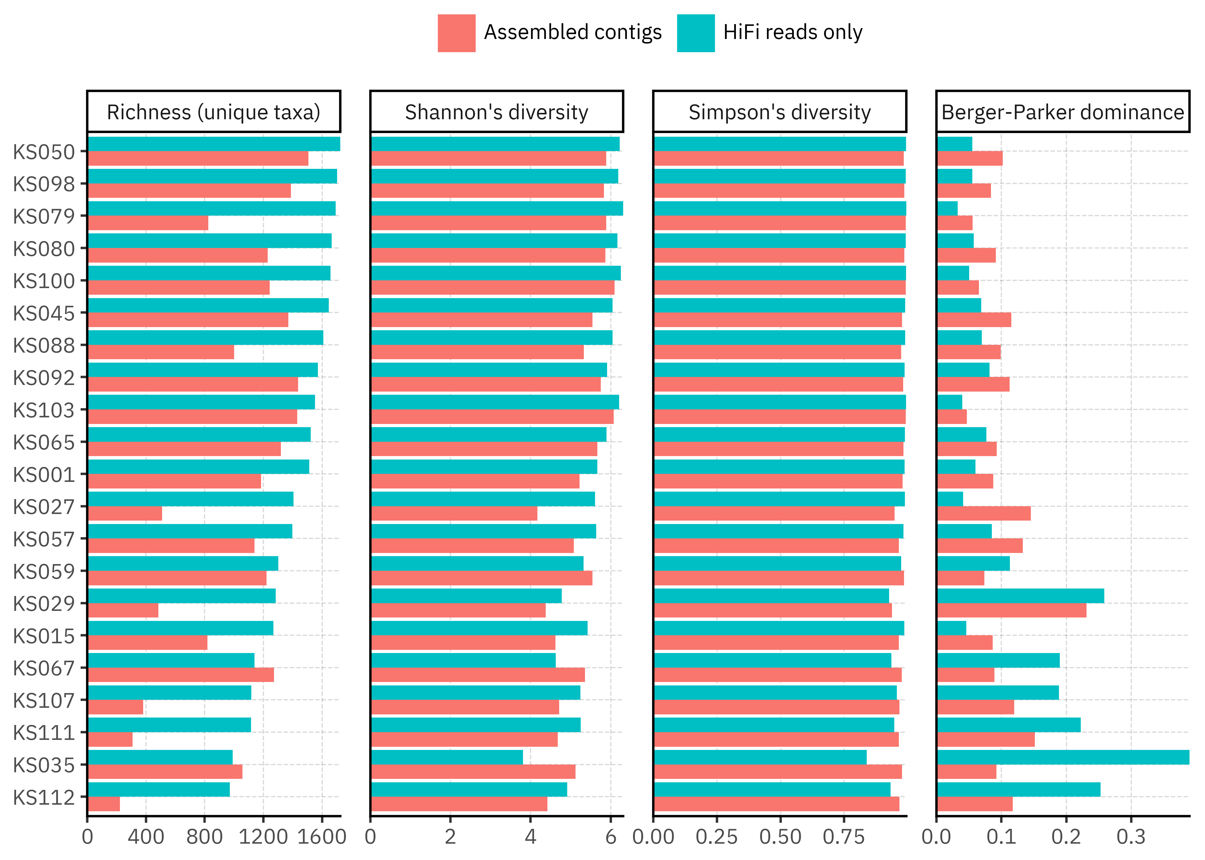
Overall, richness is consistently higher for the long-read based profiles than for the assemblies, often by a factor of 1.5–4. In contrast, Shannon and Simpson diversity are much closer between methods. This suggests that assemblies mainly prune a long tail of rare taxa while preserving the balance among the more abundant ones. A few samples (for example KS035, KS067) even show slightly higher richness in contigs, which hints that in some cases assemblies may recover taxa that direct read assignment misses, but this is not the dominant pattern.

The more detailed summary table:

Show summary table code

alpha_wide = (
    alpha_long_melted.drop(columns="kind_label")
    .query('metric_name != "Berger-Parker dominance"')
    .assign(kind=lambda dd: dd.kind.str.capitalize())
    .pivot(index="sample_id", columns=["metric_name", "kind"], values="value")
)


# Add R:C = reads / contigs for every metric
for metric in alpha_wide.columns.levels[0]:
    if metric == "Berger-Parker dominance":
        continue
    alpha_wide[(metric, "R:C")] = (
        alpha_wide[(metric, "Reads")] / alpha_wide[(metric, "Contigs")]
    )

order = ["Contigs", "Reads", "R:C"]
alpha_wide = alpha_wide.reindex(
    columns=sorted(alpha_wide.columns, key=lambda x: (x[0], order.index(x[1])))
)

tbl = alpha_wide.copy()
tbl.columns = tbl.columns.set_names(["", ""])  # instead of 'metric_name', 'kind'
tbl.index = tbl.index.set_names([""])  # instead of 'sample_id'

rich_int_cols = [
    ("Richness (unique taxa)", "Contigs"),
    ("Richness (unique taxa)", "Reads"),
]


def color_by_rich_ratio(row):
    ratio = row[("Richness (unique taxa)", "R:C")]
    if pd.isna(ratio):
        color = ""
    else:
        color = "#fdecea" if ratio < 1 else "#e6f4ea"
    return [f"background-color: {color}"] * len(row)


styled_table = (
    tbl.style.apply(color_by_rich_ratio, axis=1)
    .set_table_styles(
        [
            {"selector": "table", "props": "border-collapse: collapse;"},
            {
                "selector": "th, td",
                "props": "font-family: 'JetBrains Mono','Fira Code',monospace !important;font-size: 0.7rem;",
            },
            {
                "selector": "th.col_heading.level0",
                "props": "background-color: #333; color: white; border: 1px solid black;",
            },
            {
                "selector": "th.col_heading.level1",
                "props": "background-color: #555; color: white; border: 1px solid black;",
            },
            {
                "selector": "th.row_heading",
                "props": "background-color: #333; color: white; border: 1px solid black;",
            },
            {"selector": "tbody td", "props": "border: 1px solid #bbbbbb;"},
        ]
    )
    # default formatting: 3 decimals
    .format(precision=3)
    .format(
        lambda x: "{:,.2f}".format(x),
        subset=[
            (m, "R:C") for m in tbl.columns.levels[0] if m != "Berger-Parker dominance"
        ],
    )
    # overwrite for richness contigs/reads as integers
    .format("{:.0f}".format, subset=rich_int_cols)
)

styled_table

	Richness (unique taxa)			Shannon's diversity			Simpson's diversity
	Contigs	Reads	R:C	Contigs	Reads	R:C	Contigs	Reads	R:C

KS112	223	971	4.35	4.420	4.912	1.11	0.967	0.932	0.96
KS035	1058	990	0.94	5.119	3.809	0.74	0.978	0.839	0.86
KS111	309	1116	3.61	4.676	5.253	1.12	0.966	0.947	0.98
KS107	381	1117	2.93	4.711	5.244	1.11	0.968	0.958	0.99
KS067	1273	1140	0.90	5.356	4.630	0.86	0.977	0.936	0.96
KS015	819	1268	1.55	4.617	5.423	1.17	0.966	0.987	1.02
KS029	485	1284	2.65	4.374	4.778	1.09	0.938	0.927	0.99
KS059	1221	1302	1.07	5.547	5.320	0.96	0.985	0.974	0.99
KS057	1139	1397	1.23	5.075	5.634	1.11	0.965	0.983	1.02
KS027	510	1405	2.75	4.167	5.608	1.35	0.949	0.989	1.04
KS001	1185	1512	1.28	5.220	5.668	1.09	0.980	0.988	1.01
KS065	1319	1522	1.15	5.664	5.897	1.04	0.984	0.989	1.01
KS103	1430	1552	1.09	6.071	6.208	1.02	0.992	0.994	1.00
KS092	1437	1571	1.09	5.753	5.911	1.03	0.983	0.988	1.01
KS088	1001	1608	1.61	5.332	6.042	1.13	0.975	0.990	1.02
KS045	1370	1645	1.20	5.543	6.049	1.09	0.978	0.990	1.01
KS100	1244	1657	1.33	6.097	6.254	1.03	0.992	0.994	1.00
KS080	1229	1665	1.35	5.866	6.170	1.05	0.987	0.992	1.01
KS079	824	1693	2.05	5.886	6.313	1.07	0.992	0.995	1.00
KS098	1388	1702	1.23	5.830	6.188	1.06	0.987	0.993	1.01
KS050	1507	1724	1.14	5.889	6.226	1.06	0.985	0.993	1.01

The summary table makes this clearer. For almost all samples the richness ratio (Reads / Contigs) is above 1, sometimes well above, while the corresponding ratios for Shannon and Simpson cluster close to 1. In practical terms, assemblies tend to reduce the number of reported taxa without collapsing the community into a few dominant groups. This is reassuring for downstream ecological interpretation, but it also flags that any analysis focused on rare taxa will be sensitive to the choice of pipeline.

Beta-diversity comparison

If we go ahead and compute the Bray-Curtis distance between all possible pairs of samples, we obtain the following matrix:

Show Code

df_wide = (
    tax_dfs.groupby(["sample_id", "kind", "taxid"])["count"]
    .sum()
    .unstack("taxid", fill_value=0)
)
(
    df_wide.reset_index()
    .assign(sample_code=lambda dd: dd["sample_id"] + "_" + dd["kind"])
    .drop(columns=["sample_id", "kind"])
    .set_index("sample_code")
    .T.corr(method=braycurtis)
    .reset_index()
    .assign(sample_x=lambda dd: dd["sample_code"].str.split("_").str[0])
    .assign(kind_x=lambda dd: dd["sample_code"].str.split("_").str[1])
    .drop(columns="sample_code")
    .melt(id_vars=["sample_x", "kind_x"])
    .assign(sample_y=lambda dd: dd["sample_code"].str.split("_").str[0])
    .assign(kind_y=lambda dd: dd["sample_code"].str.split("_").str[1])
    .drop(columns="sample_code")
    .query("~(sample_x == sample_y & kind_x == kind_y)")
    .pipe(
        lambda dd: p9.ggplot(dd)
        + p9.aes(
            x="sample_x + kind_x.str.capitalize().str[0]",
            y="sample_y + kind_y.str.capitalize().str[0]",
            fill="value",
        )
        + p9.geom_tile()
        + p9.labs(
            x="",
            y="",
            fill="Bray-Curtis distance",
            caption="*Using total counts for Bray-Curtis distance",
        )
        + p9.scale_x_discrete(expand=(0, 0))
        + p9.scale_y_discrete(expand=(0, 0))
        + p9.theme(
            figure_size=(6, 6),
            axis_text=p9.element_text(family="monospace", size=8),
            axis_text_x=p9.element_text(rotation=90),
            panel_grid=p9.element_blank(),
            panel_background=p9.element_rect(fill="#545353"),
            legend_position="top",
            legend_frame=p9.element_rect(),
            legend_key_height=17.5,
            plot_caption=p9.element_text(margin={"t": 10}),
        )
    )
)

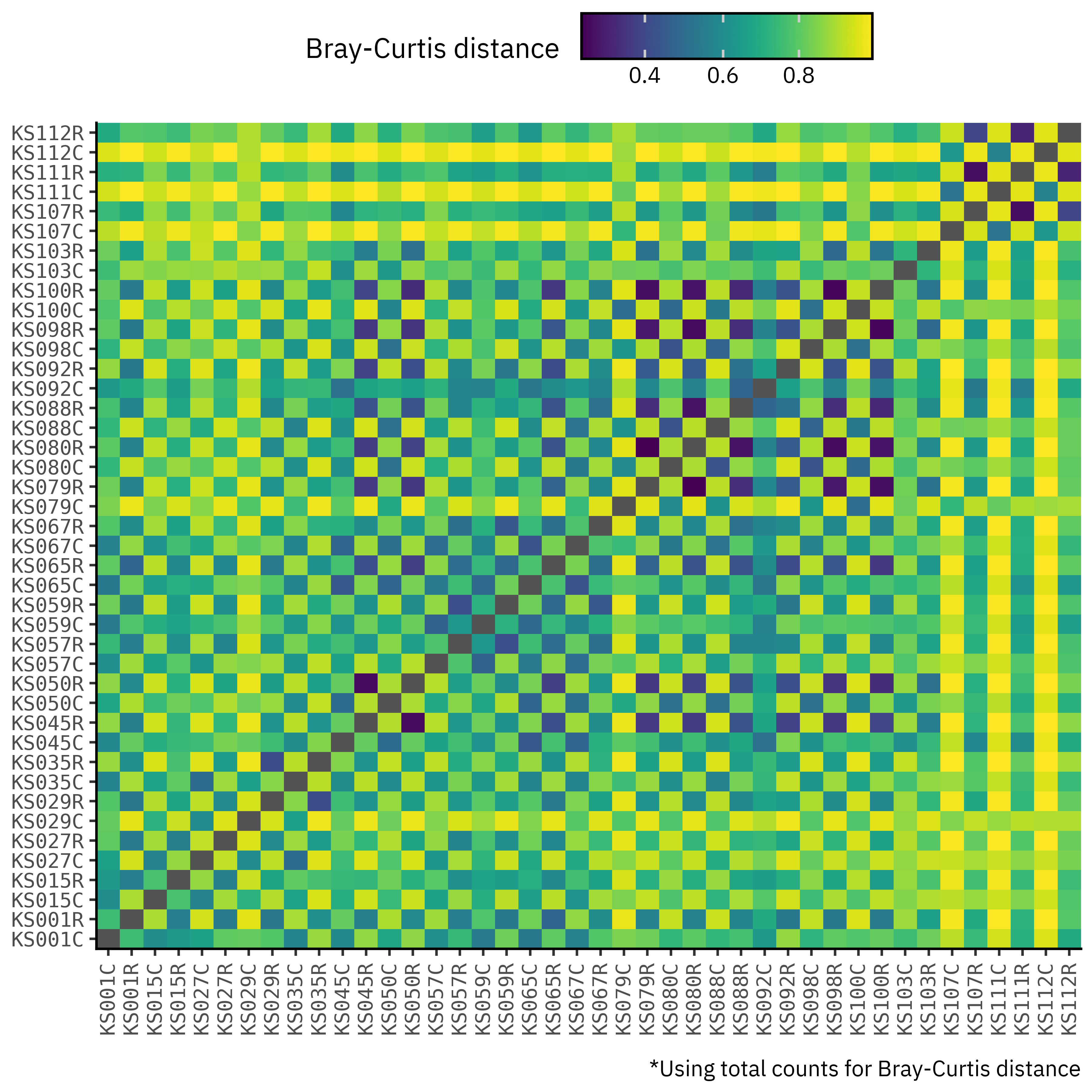
Weird, right? Well of course, it’s because we’re comparing assemblies with long reads, with total counts being in completely different scales and so we get this weird checkerboard pattern because contig samples will always be closer to each other than to unassembled samples just based on the total counts of each method.

To do a proper assessment, then, we need to normalize the counts, and so we will use the relative abundances of each taxon in each sample as a proxy for the true relative abundances and to compute Bray-Curtis distances:

Show Code

df_wide_rel = (
    tax_dfs
    # compute per sample relative abundance
    .groupby(["sample_id", "kind"], as_index=False)
    .apply(lambda dd: dd.assign(ra=dd["count"] / dd["count"].sum()))
    .groupby(["sample_id", "kind", "taxid"])["ra"]
    .sum()
    .unstack("taxid", fill_value=0)
)
dist_mat_rel = (
    df_wide_rel.reset_index()
    .assign(sample_code=lambda dd: dd["sample_id"] + "_" + dd["kind"])
    .drop(columns=["sample_id", "kind"])
    .set_index("sample_code")
    .T.corr(method=braycurtis)
)

bc_rel_long = (
    dist_mat_rel.reset_index()
    .assign(sample_x=lambda dd: dd["sample_code"].str.split("_").str[0])
    .assign(kind_x=lambda dd: dd["sample_code"].str.split("_").str[1])
    .drop(columns="sample_code")
    .melt(id_vars=["sample_x", "kind_x"])
    .assign(sample_y=lambda dd: dd["sample_code"].str.split("_").str[0])
    .assign(kind_y=lambda dd: dd["sample_code"].str.split("_").str[1])
    .drop(columns="sample_code")
    .query("~(sample_x == sample_y & kind_x == kind_y)")
)


(
    bc_rel_long.pipe(
        lambda dd: p9.ggplot(dd)
        + p9.aes(
            x="sample_x + kind_x.str.capitalize().str[0]",
            y="sample_y + kind_y.str.capitalize().str[0]",
            fill="value",
        )
        + p9.geom_tile()
        + p9.labs(
            x="",
            y="",
            fill="Bray-Curtis distance",
            caption="*Using relative abundance for Bray-Curtis distance",
        )
        + p9.scale_x_discrete(expand=(0, 0))
        + p9.scale_y_discrete(expand=(0, 0))
        + p9.theme(
            figure_size=(6, 6),
            axis_text=p9.element_text(family="monospace", size=8),
            axis_text_x=p9.element_text(rotation=90),
            panel_grid=p9.element_blank(),
            panel_background=p9.element_rect(fill="#545353"),
            legend_position="top",
            legend_frame=p9.element_rect(),
            legend_key_height=17.5,
            plot_caption=p9.element_text(margin={"t": 10}),
        )
    )
)

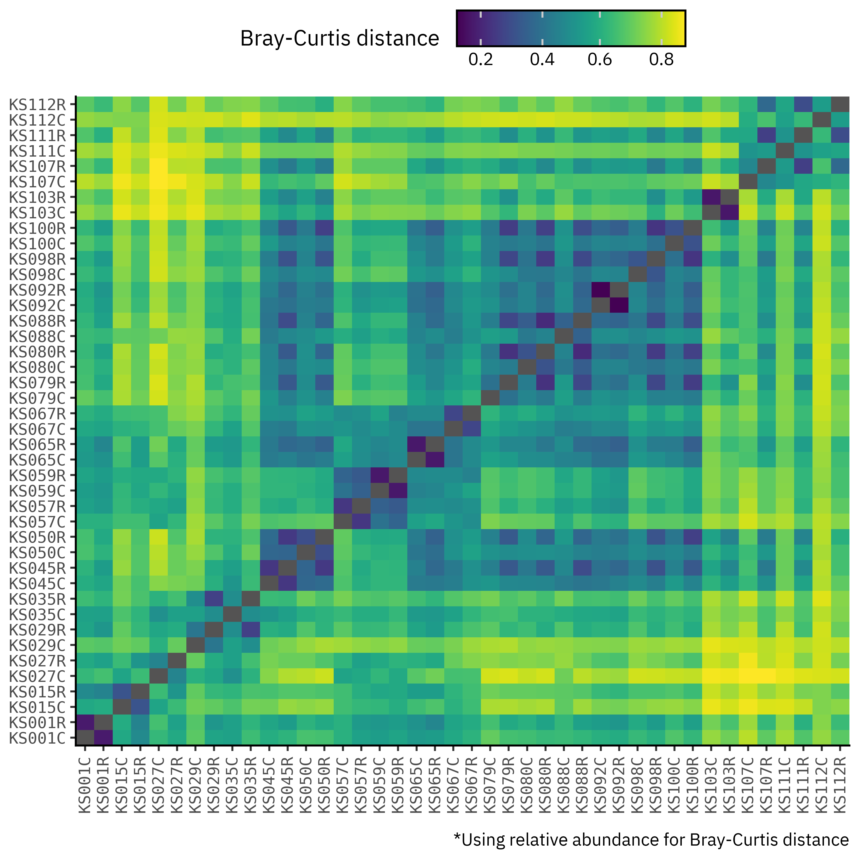
Once we switch to relative abundances, the structure of the matrix changes. Blocks corresponding to contigs vs reads become much less contrasted, and off-diagonal cells no longer show a strict contig-to-contig vs read-to-read separation. Distances between profiles from the same sample are now comparable in magnitude to distances between different samples, which tells us that after controlling for library size, the pipelines are capturing broadly similar communities with sample identity still being the main source of variation.

Distance grouping calculations

read_contigs_distances = (
    bc_rel_long.query("sample_x == sample_y")
    .query('kind_x == "reads"')
    .rename(columns={"sample_x": "sample"})[["sample", "value"]]
    .assign(label="Reads ↔ Contigs")
)

read_reads_distances = (
    bc_rel_long.query("sample_x != sample_y")
    .query('kind_x == "reads"')
    .query('kind_y == "reads"')
    .groupby("sample_x", as_index=False)
    .agg(value=("value", "mean"))
    .rename(columns={"sample_x": "sample"})
    .assign(label="Reads → Other reads")
)

contig_contig_distances = (
    bc_rel_long.query("sample_x != sample_y")
    .query('kind_x == "contigs"')
    .query('kind_y == "contigs"')
    .groupby("sample_x", as_index=False)
    .agg(value=("value", "mean"))
    .rename(columns={"sample_x": "sample"})
    .assign(label="Contigs → Other contigs")
)

contig_read_distances = (
    bc_rel_long.query("sample_x != sample_y")
    .query('kind_x == "contigs"')
    .query('kind_y == "reads"')
    .groupby("sample_x", as_index=False)
    .agg(value=("value", "mean"))
    .rename(columns={"sample_x": "sample"})
    .assign(label="Contigs → Other reads")
)

all_distances = pd.concat(
    [
        read_contigs_distances,
        read_reads_distances,
        contig_read_distances,
        contig_contig_distances,
    ]
)

Show Code

samples_order = read_contigs_distances.sort_values(by="value")["sample"]
label_order = all_distances.label.unique()
label_order = label_order[::-1]
(
    all_distances.assign(
        sample=lambda dd: pd.Categorical(
            dd["sample"], categories=samples_order, ordered=True
        )
    )
    .assign(
        label=lambda dd: pd.Categorical(
            dd["label"], categories=label_order, ordered=False
        )
    )
    .pipe(
        lambda dd: p9.ggplot(dd)
        + p9.aes(y="sample", x="value")
        + p9.geom_segment(
            p9.aes(yend="sample", xend="value", x=0, color="label"),
            size=0.8,
            arrow=p9.arrow(angle=30, length=0.095, type="closed"),
        )
        + p9.scale_x_continuous(limits=(0, 1), expand=(0, 0))
        + p9.scale_color_manual(["#D3894C", "#435B97", "#ab2422", "#32a86d"])
        + p9.labs(x="Bray-Curtis distance", y="", color="")
        + p9.guides(color=p9.guide_legend(ncol=2))
        + p9.theme(
            figure_size=(3.5, 4),
            axis_text_y=p9.element_text(family="monospace", size=8),
            axis_title_x=p9.element_text(size=10),
            legend_text=p9.element_text(size=6, family="monospace"),
            legend_key_size=10,
            legend_position="top",
        )
    )
)

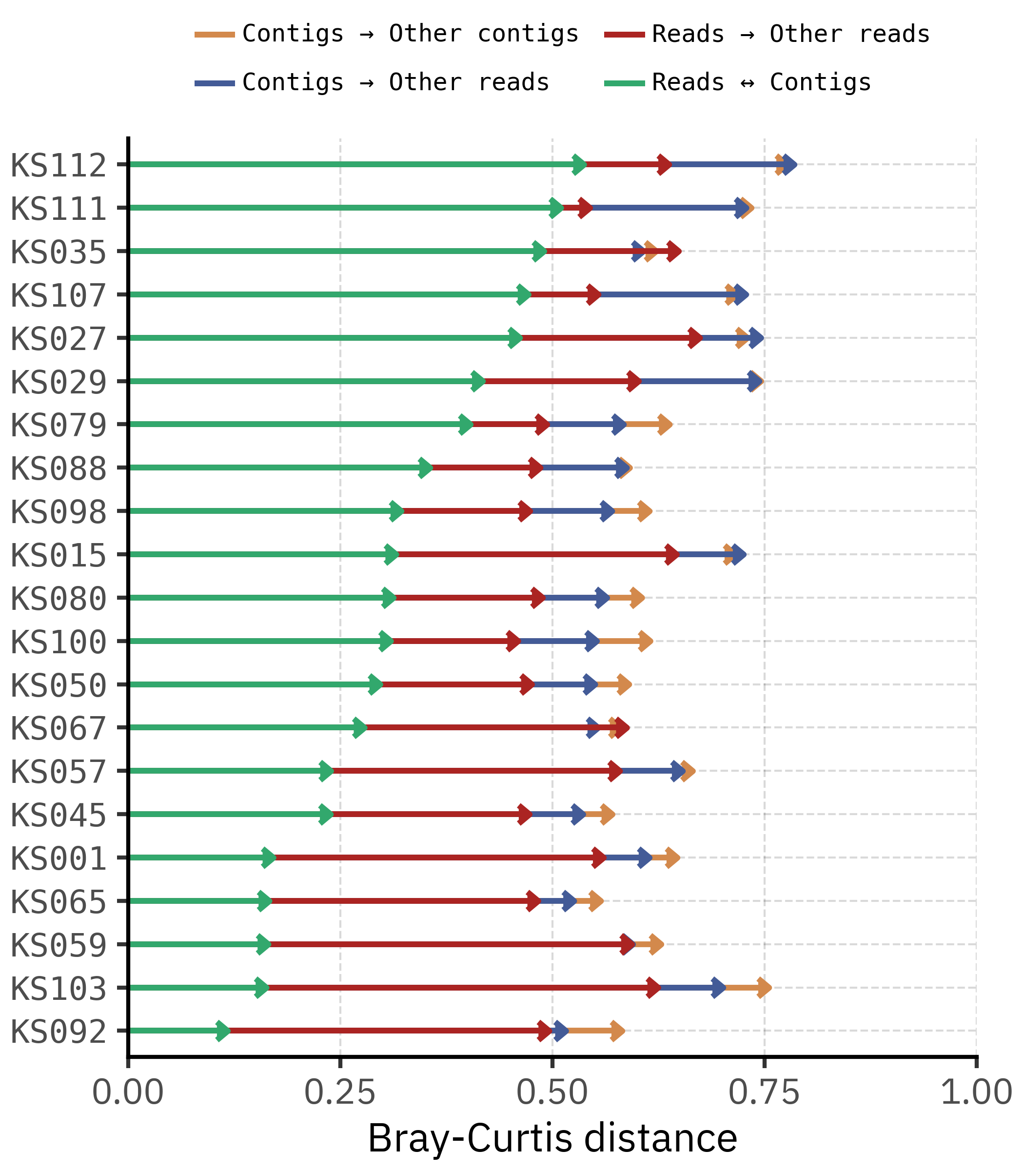
The segment plot helps disentangle within-sample and between-sample distances. For each sample, we compare four quantities: the distance between reads and contigs of the same sample, the mean distance from reads to other read profiles, the mean distance from contigs to other contig profiles, and the cross-comparison between contigs and reads from other samples.

In most cases the Reads ↔︎ Contigs arrow lies well to the left of the arrows that connect to other samples. This means that, for a given sample, the contig profile is closer to its own read profile than to any other sample’s community. The method effect is therefore smaller than the between-sample effect, consistent with the PCoA and PERMANOVA results.

Show Code

(
    all_distances.assign(
        label=lambda dd: dd.label.str.replace("Other", "\nOther")
    ).pipe(
        lambda dd: p9.ggplot(dd)
        + p9.aes("label", y="value", fill="label")
        + p9.geom_jitter(
            stroke=0,
            width=0.1,
            size=2,
        )
        + p9.geom_boxplot(alpha=0.5)
        + p9.labs(x="", y="Bray-Curtis distance")
        + p9.scale_fill_manual(["#D3894C", "#435B97", "#ab2422", "#32a86d"])
        + p9.scale_y_continuous(limits=(0, 1), expand=(0, 0))
        + p9.guides(fill=False)
        + p9.theme(
            figure_size=(4, 2.5),
            axis_text_x=p9.element_text(family="monospace", size=7),
        )
    )
)

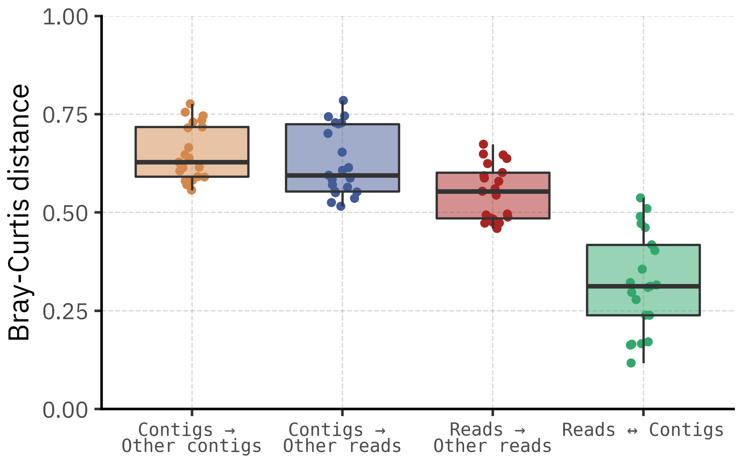
Aggregating across samples, the distribution of Bray–Curtis distances confirms this pattern. Distances between reads and contigs from the same sample are shifted towards lower values compared with distances between unrelated samples, regardless of whether we compare reads to reads, contigs to contigs, or contigs to reads. There is still some overlap, which reflects both biological similarity among certain samples and noise from low abundance taxa, but the central tendency is clear: most of the time the two pipelines agree more with each other than with any other sample.

Impact of assembly on community composition estimates

Let’s now use the Bray-Curtis distances derived from the relative abundances to perform a PCoA of the taxonomic profiles and run a PERMANOVA to test for significant differences between the assemblies and the long HiFi reads.

We’ll use R’s vegan package to compute the PERMANOVA, as we will compare the contigs vs long HiFi reads groups both globally and adjusted for paired samples, that is, do we see a difference in the communities of contigs vs long HiFi reads even when we control for the individual samples?

Wrangling for permanova

meta_df = df_wide_rel.reset_index()[["sample_id", "kind"]].assign(
    id=lambda dd: dd["sample_id"] + "_" + dd["kind"]
)

abund_only = df_wide_rel.reset_index(drop=True)

%%R -i abund_only -i meta_df


# Use the combined id as rownames so community and metadata match
rownames(abund_only) <- meta_df$id

# Unpaired PERMANOVA: no blocking, just test kind (reads vs contigs)
adon_unpaired <- adonis2(
  abund_only ~ kind,
  data = meta_df,
  method = "bray",
  permutations = 999
)

# Paired PERMANOVA: same model, but permutations restricted by sample_id
adon_paired <- adonis2(
  abund_only ~ kind,
  data = meta_df,
  method = "bray",
  permutations = 999,
  strata = meta_df$sample_id
)

print(adon_unpaired)
print(adon_paired)

Permutation test for adonis under reduced model
Permutation: free
Number of permutations: 999

adonis2(formula = abund_only ~ kind, data = meta_df, permutations = 999, method = "bray")
         Df SumOfSqs      R2      F Pr(>F)  
Model     1   0.3255 0.04092 1.7067  0.051 .
Residual 40   7.6297 0.95908                
Total    41   7.9552 1.00000                
---
Signif. codes:  0 ‘***’ 0.001 ‘**’ 0.01 ‘*’ 0.05 ‘.’ 0.1 ‘ ’ 1
Permutation test for adonis under reduced model
Blocks:  strata 
Permutation: free
Number of permutations: 999

adonis2(formula = abund_only ~ kind, data = meta_df, permutations = 999, method = "bray", strata = meta_df$sample_id)
         Df SumOfSqs      R2      F Pr(>F)    
Model     1   0.3255 0.04092 1.7067  0.001 ***
Residual 40   7.6297 0.95908                  
Total    41   7.9552 1.00000                  
---
Signif. codes:  0 ‘***’ 0.001 ‘**’ 0.01 ‘*’ 0.05 ‘.’ 0.1 ‘ ’ 1

PCoA computation and plot code

X = df_wide_rel.values  # samples × taxa
ids = [f"{sid}_{kind}" for sid, kind in df_wide_rel.index]
bc = beta_diversity("braycurtis", X, ids=ids)
pcoa_res = pcoa(bc)
coords = pcoa_res.samples
coords["sample_id"] = [sid for sid, kind in df_wide_rel.index]
coords["kind"] = [kind.capitalize() for sid, kind in df_wide_rel.index]

# Now we compute some segments to show the paired nature of the comparison in the plot
seg = coords.pivot(
    index="sample_id", columns="kind", values=["PC1", "PC2"]
).reset_index()

seg.columns = [
    "sample_id",
    "PC1_contigs",
    "PC1_reads",
    "PC2_contigs",
    "PC2_reads",
]

segments = pd.DataFrame(
    {
        "sample_id": seg["sample_id"],
        "x": seg["PC1_reads"],
        "y": seg["PC2_reads"],
        "xend": seg["PC1_contigs"],
        "yend": seg["PC2_contigs"],
    }
)


(
    p9.ggplot(coords)
    + p9.aes(x="PC1", y="PC2", color="kind")
    + p9.geom_segment(
        data=segments,
        linetype="dashed",
        mapping=p9.aes(x="x", y="y", xend="xend", yend="yend"),
        alpha=0.5,
        size=0.9,
        inherit_aes=False,
    )
    + p9.geom_point()
    + p9.scale_x_continuous(expand=(0.075, 0.075))
    + p9.scale_y_continuous(expand=(0.075, 0.075))
    + p9.geom_rug(size=0.5)
    + p9.labs(
        color="",
        caption="PERMANOVA p-value: unpaired: 0.057, paired: 0.001",
        x="PCo1",
        y="PCo2",
    )
    + p9.theme(
        figure_size=(5, 4),
        legend_position="top",
        plot_caption=p9.element_text(margin={"t": 10, "r": 5}),
    )
)

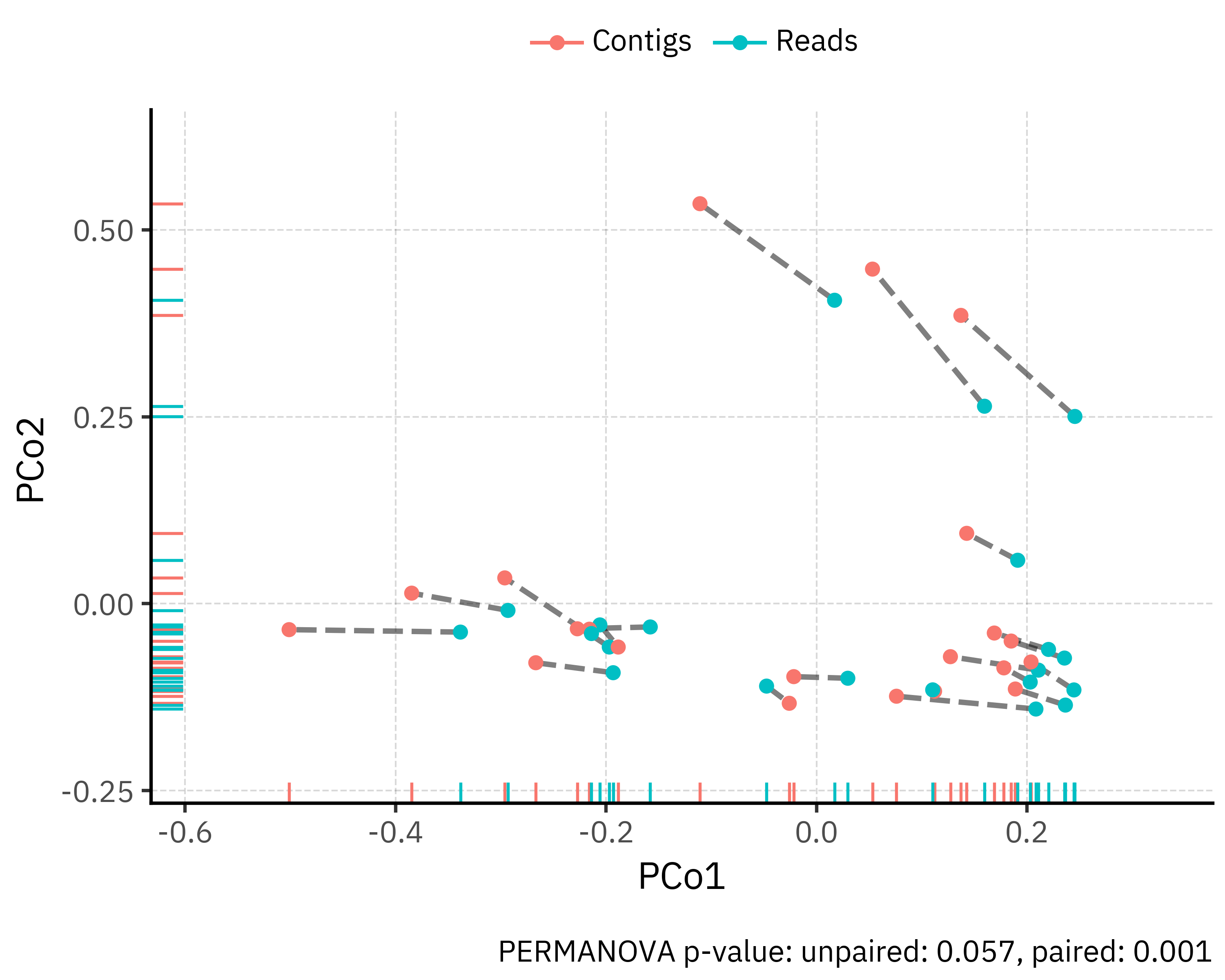
The PCoA plot shows that community composition is driven mainly by between-sample differences rather than by the processing method. Each point is one profile (reads or contigs) and paired profiles from the same sample are linked by a dashed segment. Most segments are short compared with the overall spread of points, so reads and contigs from the same sample occupy nearby positions in ordination space.

We quantified the method effect with PERMANOVA on Bray-Curtis distances:

Unpaired PERMANOVA (kind only): R² = 0.041, p = 0.057
Paired PERMANOVA (permutations restricted within sample_id): R² = 0.041, p = 0.001

In both cases the effect size of kind is small (about 4 % of variance), confirming that most of the structure in the data is sample specific. The difference between p-values reflects the design: when sample identity is ignored, the modest method effect is hard to distinguish from overall between-sample variation. Once we constrain permutations within each sample, we test only the within-sample shift from reads to contigs and detect a consistent, statistically significant but subtle change in composition across samples.

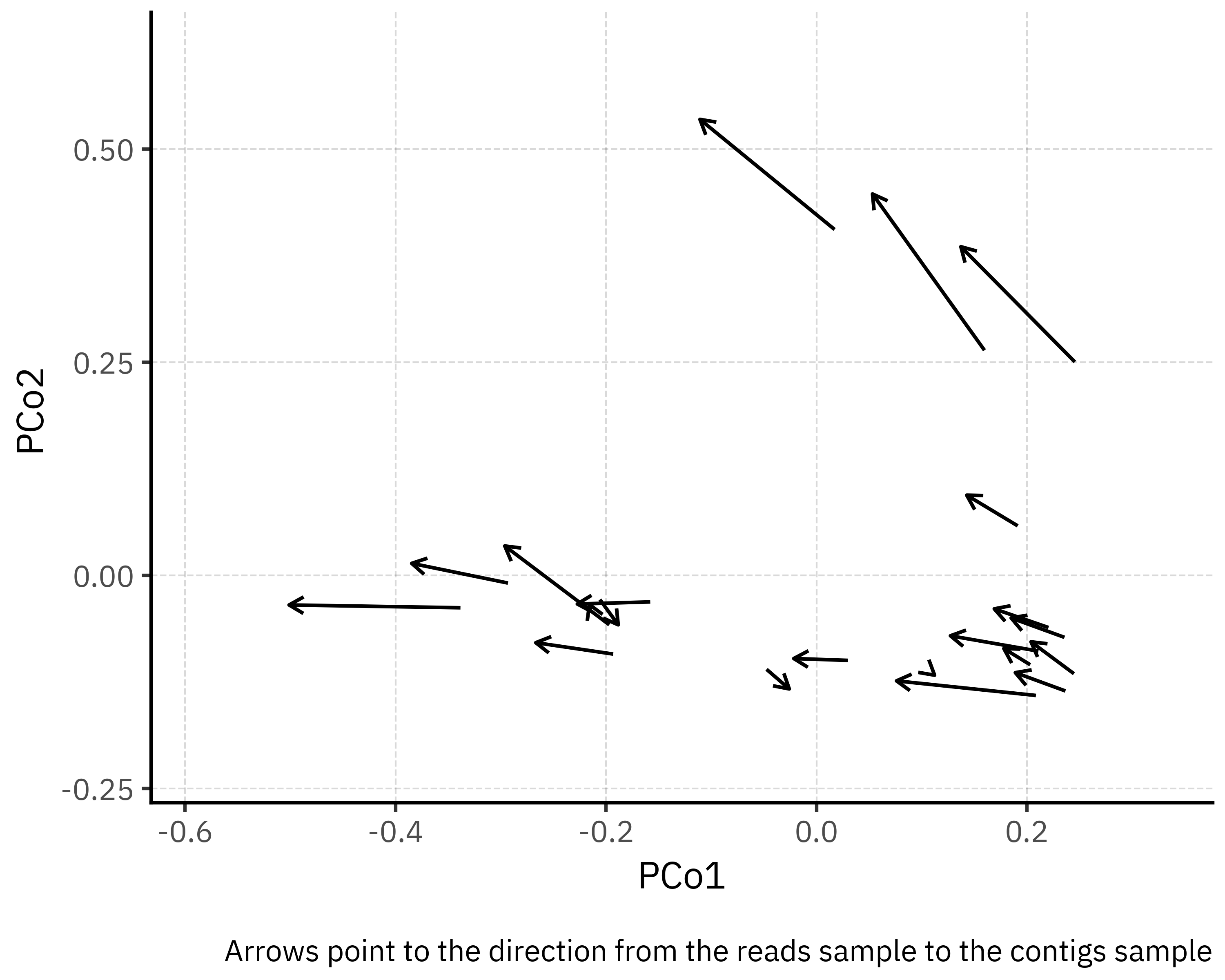
One caveat is that PERMANOVA is sensitive to differences in multivariate dispersion between groups. Here, visual inspection of the PCoA suggests that contigs and reads have comparable spread, so the small but significant effect detected in the paired design is most likely due to a genuine shift in centroids rather than inflated by dispersion. In any case, the effect size remains modest. From a practical point of view, assemblies do shift community composition in a consistent direction (see the plot below showcasing only the projected shift from reads to contigs in each sample, with a consistent leftward shift), but the magnitude of that shift is small relative to the ecological differences between samples.

Show Code

(
    p9.ggplot(segments)
    + p9.geom_segment(
        data=segments,
        linetype="solid",
        mapping=p9.aes(x="x", y="y", xend="xend", yend="yend"),
        alpha=1,
        size=0.6,
        arrow=p9.arrow(length=0.1),
        inherit_aes=False,
    )
    + p9.scale_x_continuous(expand=(0.075, 0.075))
    + p9.scale_y_continuous(expand=(0.075, 0.075))
    + p9.labs(
        color="",
        caption="Arrows point to the direction from the reads sample to the contigs sample",
        x="PCo1",
        y="PCo2",
    )
    + p9.theme(
        figure_size=(5, 4),
        legend_position="top",
        plot_caption=p9.element_text(margin={"t": 10, "r": 5}),
    )
)

Focusing on the differences

In the previous section we saw that assemblies introduce a small but consistent shift in community composition, while most of the structure is still driven by sample identity. To understand what this means biologically, we now zoom in on the actual taxa where the pipelines disagree: which taxa are found only in reads, which are only in contigs, and how much of the total community they represent.

The goal is to separate two possibilities. Either (i) the differences are mainly a cloud of low abundance or strain-level taxa at the bottom of the distribution, in which case both pipelines tell the same ecological story, or (ii) the differences involve substantial fractions of abundant taxa, which would mean that the choice of pipeline can change our conclusions about which organisms dominate the aerobiome.

Taxa differences wrangling

differences_dict = defaultdict(dict)
for sample_id, df in df_wide_rel.groupby(level=0):
    reads_set = set(df.loc[sample_id, "reads"].loc[lambda x: x > 0].index.to_list())
    contigs_set = set(df.loc[sample_id, "contigs"].loc[lambda x: x > 0].index.to_list())
    shared = reads_set & contigs_set
    reads_only = reads_set - shared
    contigs_only = contigs_set - shared
    full_set = reads_set | contigs_set
    shared_fraction = len(shared) / len(full_set)
    shared_total = len(shared)
    contigs_only_total = len(contigs_only)
    reads_only_total = len(reads_only)
    reads_only_fraction = len(reads_only) / len(full_set)
    contigs_only_fraction = len(contigs_only) / len(full_set)
    shared_weight_reads = float(df.loc[sample_id, "reads"].loc[list(shared)].sum())
    shared_weight_contigs = float(df.loc[sample_id, "contigs"].loc[list(shared)].sum())
    reads_only_weight = float(df.loc[sample_id, "reads"].loc[list(reads_only)].sum())
    contigs_only_weight = float(
        df.loc[sample_id, "contigs"].loc[list(contigs_only)].sum()
    )
    differences_dict[sample_id] = {
        "shared_fraction": shared_fraction,
        "reads_only_fraction": reads_only_fraction,
        "contigs_only_fraction": contigs_only_fraction,
        "shared_weight_reads": shared_weight_reads,
        "shared_weight_contigs": shared_weight_contigs,
        "reads_only_weight": reads_only_weight,
        "contigs_only_weight": contigs_only_weight,
        "shared_total": shared_total,
        "contigs_only_total": contigs_only_total,
        "reads_only_total": reads_only_total,
    }

diff_df = pd.DataFrame(differences_dict).T
diff_df.index.name = "sample_id"
diff_df = diff_df.reset_index()

taxa_cols = ["shared_fraction", "reads_only_fraction", "contigs_only_fraction"]

weight_cols = [
    "shared_weight_reads",
    "reads_only_weight",
    "shared_weight_contigs",
    "contigs_only_weight",
]

taxa_long = diff_df.melt(
    id_vars="sample_id",
    value_vars=taxa_cols,
    var_name="region",
    value_name="fraction",
)

region_labels = {
    "shared_fraction": "Shared",
    "reads_only_fraction": "Reads only",
    "contigs_only_fraction": "Contigs only",
}
taxa_long["region"] = taxa_long["region"].map(region_labels)

# order samples by shared_fraction if you like
order = diff_df.sort_values("shared_fraction")["sample_id"].tolist()
taxa_long["sample_id"] = pd.Categorical(
    taxa_long["sample_id"], categories=order, ordered=True
)

wdf = diff_df.rename(
    columns={
        "shared_weight_reads": "reads_shared",
        "reads_only_weight": "reads_only",
        "shared_weight_contigs": "contigs_shared",
        "contigs_only_weight": "contigs_only",
    }
)

weight_long = wdf.melt(
    id_vars="sample_id",
    value_vars=["reads_shared", "reads_only", "contigs_shared", "contigs_only"],
    var_name="metric",
    value_name="weight",
)

# split into method and region
method_region = weight_long["metric"].str.split("_", n=1, expand=True)
weight_long["method"] = method_region[0].str.capitalize()
weight_long["region"] = method_region[1].map({"shared": "Shared", "only": "Unique"})

# use same sample order as before
weight_long["sample_id"] = pd.Categorical(
    weight_long["sample_id"], categories=order, ordered=True
)
weight_long["metric"] = weight_long["metric"].map(
    {
        "reads_shared": "Shared",
        "contigs_shared": "Shared",
        "reads_only": "Reads only",
        "contigs_only": "Contigs only",
    }
)

Show Code

p_taxa = (
    p9.ggplot(taxa_long, p9.aes("sample_id", "fraction", fill="region"))
    + p9.geom_col()
    + p9.coord_flip()
    + p9.scale_y_continuous(
        labels=percent_format(), expand=(0, 0), breaks=[0, 0.25, 0.5, 0.75]
    )
    + p9.geom_text(
        p9.aes(label="shared_total.astype(int)", x="sample_id"),
        inherit_aes=False,
        y=0.01,
        ha="left",
        size=6,
        family="monospace",
        color="white",
        data=diff_df,
    )
    + p9.geom_text(
        p9.aes(label="contigs_only_total.astype(int)", x="sample_id"),
        inherit_aes=False,
        y=0.995,
        ha="right",
        size=6,
        family="monospace",
        color="white",
        data=diff_df,
    )
    + p9.geom_text(
        p9.aes(
            label="reads_only_total.astype(int)",
            x="sample_id",
            y="shared_fraction + reads_only_fraction / 2",
        ),
        inherit_aes=False,
        ha="left",
        nudge_y=-0.03,
        size=6,
        family="monospace",
        color="white",
        data=diff_df,
    )
    + p9.scale_fill_manual(
        values=["#D3894C", "#435B97", "#ab2422"],
        breaks=["Shared", "Contigs only", "Reads only"],
    )
    + p9.labs(
        x="",
        y="Fraction of unique taxa",
        fill="",
        title="",
    )
    + p9.theme(
        legend_position=(0.5, 1.075),
        legend_direction="horizontal",
        axis_text_y=p9.element_text(family="monospace", size=7),
        legend_key_size=9,
        plot_margin_right=0,
        axis_text_x=p9.element_text(size=7),
    )
)

p_weight = (
    p9.ggplot(weight_long, p9.aes("sample_id", "weight", fill="metric"))
    + p9.geom_col()
    + p9.coord_flip()
    + p9.scale_y_continuous(
        labels=percent_format(), expand=(0, 0), breaks=[0, 0.25, 0.5, 0.75]
    )
    + p9.scale_fill_manual(
        values=["#D3894C", "#435B97", "#ab2422"],
        breaks=["Shared", "Contigs only", "Reads only"],
    )
    + p9.facet_wrap("~method", nrow=1)
    + p9.labs(
        x="",
        y="Fraction of abundance",
        fill="",
        title="",
    )
    + p9.guides(fill=False)
    + p9.theme(
        figure_size=(6, 4),
        axis_text_y=p9.element_blank(),
        axis_ticks_y=p9.element_blank(),
        axis_text_x=p9.element_text(size=7),
        plot_margin_left=0,
    )
)

p_taxa | p_weight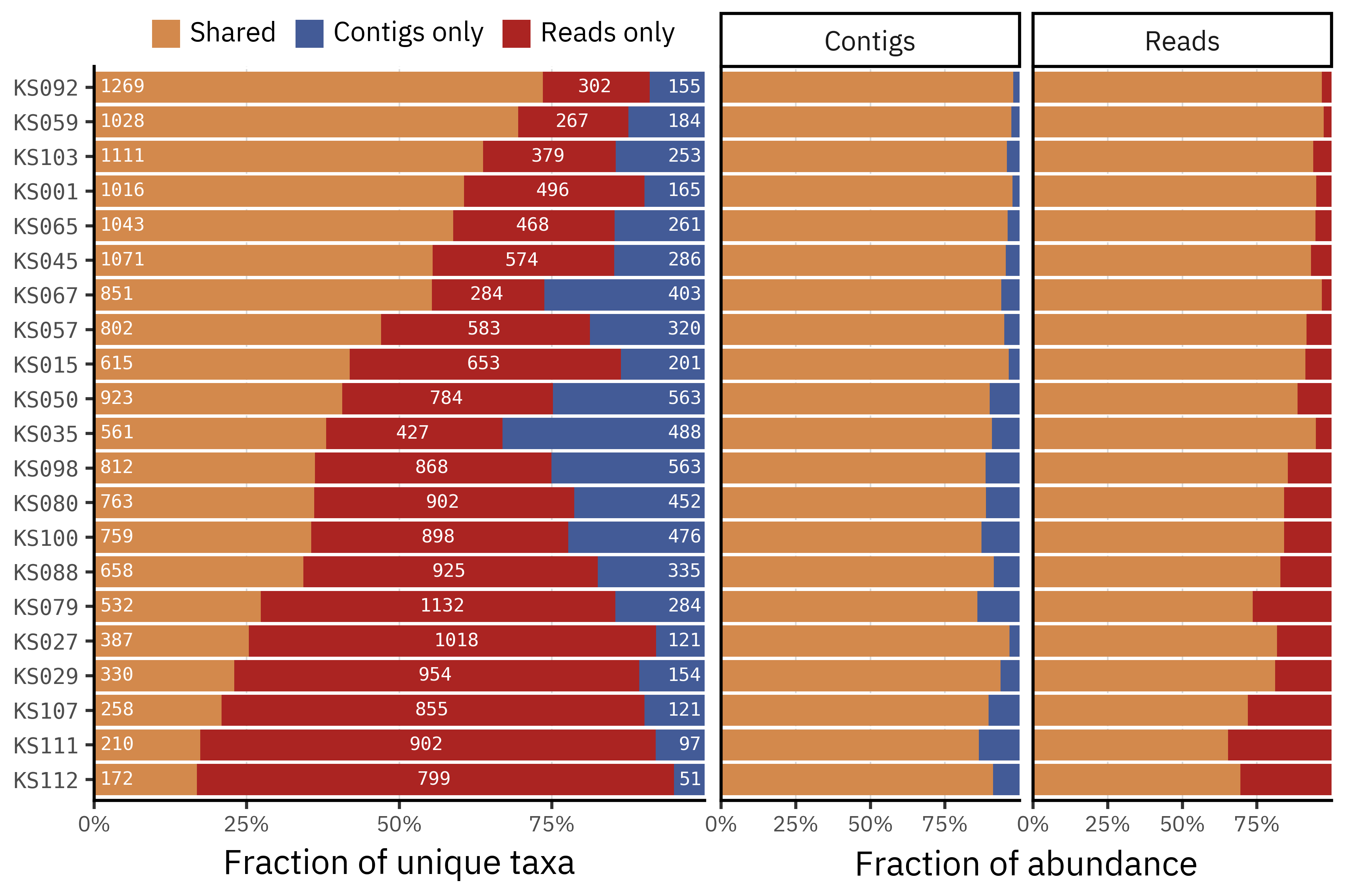

Each bar on the left splits the taxa detected in a given sample into three groups: taxa shared by both pipelines (orange), taxa only detected in reads (red), and taxa only detected in contigs (blue). The numbers inside the segments indicate the absolute number of taxa in each group. Across samples it is common for 40–80 % of taxa to be unique to a single pipeline, and this uniqueness is usually skewed towards reads rather than contigs.

The right panels repeat the exercise but now for relative abundance, weighting taxa by how abundant they are in each method. Here the picture is very different: for both pipelines more than 80–90 % of the total abundance lies in taxa that are shared between assemblies and non-assemblies, with only a small fraction of reads or contigs assigned to taxa that are unique to one method. This indicates that most disagreements concern low-abundance taxa or fine strain level splits, while the dominant community structure is largely preserved. The choice of pipeline should therefore matter most for analyses that focus on rare taxa, such as detection of specific pathogens or strain-level tracking.

Show Code

mean_rel_df = df_wide_rel.groupby("kind").mean()
reads_set = set(mean_rel_df.loc["reads"].loc[lambda x: x > 0].index.values)
contigs_set = set(mean_rel_df.loc["contigs"].loc[lambda x: x > 0].index.values)

only_reads = reads_set - contigs_set
only_contigs = contigs_set - reads_set
shared = reads_set & contigs_set
union = reads_set | contigs_set

mean_only_contigs_abundance = mean_rel_df.loc["contigs"].loc[list(only_contigs)].sum()
mean_only_reads_abundance = mean_rel_df.loc["reads"].loc[list(only_reads)].sum()
mean_shared_contigs_abundance = 1 - mean_only_contigs_abundance
mean_shared_reads_abundance = 1 - mean_only_reads_abundance

global_taxa = pd.DataFrame(
    {
        "sample_id": ["All samples"] * 3,
        "region": ["Shared", "Contigs only", "Reads only"],
        "fraction": [
            len(shared) / len(union),
            len(only_contigs) / len(union),
            len(only_reads) / len(union),
        ],
        "n_taxa": [len(shared), len(only_contigs), len(only_reads)],
    }
)

global_rel_ab = pd.DataFrame(
    {
        "sample_id": ["All samples"] * 4,
        "region": ["Shared", "Contigs only", "Shared", "Reads only"],
        "method": ["Contigs", "Contigs", "Reads", "Reads"],
        "weight": [
            mean_shared_contigs_abundance,
            mean_only_contigs_abundance,
            mean_shared_reads_abundance,
            mean_only_reads_abundance,
        ],
    }
)


p_global_taxa = (
    p9.ggplot(global_taxa, p9.aes("sample_id", "fraction", fill="region"))
    + p9.geom_col()
    # numbers of taxa inside each coloured segment
    + p9.geom_text(
        p9.aes(label="n_taxa"),
        position=p9.position_stack(vjust=0.5),
        size=7,
        color="white",
        family="monospace",
    )
    + p9.coord_flip()
    + p9.scale_y_continuous(labels=percent_format(), expand=(0, 0))
    + p9.scale_fill_manual(
        values=["#D3894C", "#435B97", "#ab2422"],
        breaks=["Shared", "Contigs only", "Reads only"],
    )
    + p9.labs(
        x="",
        y="Fraction of unique taxa",
        fill="",
        title="",
    )
    + p9.guides(fill=False)
    + p9.theme(
        axis_text_x=p9.element_text(size=7),
    )
)

p_global_rel_ab = (
    p9.ggplot(global_rel_ab, p9.aes("sample_id", "weight", fill="region"))
    + p9.geom_col()
    + p9.geom_text(
        p9.aes(label="(weight * 100).round(2).astype(str) + '%'"),
        position=p9.position_stack(vjust=0.5),
        size=7,
        color="white",
        family="monospace",
        data=global_rel_ab.query('region == "Shared"'),
    )
    + p9.coord_flip()
    + p9.scale_y_continuous(
        labels=percent_format(), expand=(0, 0), breaks=[0, 0.25, 0.5, 0.75]
    )
    + p9.scale_fill_manual(
        values=["#D3894C", "#435B97", "#ab2422"],
        breaks=["Shared", "Contigs only", "Reads only"],
    )
    + p9.facet_wrap("~method", nrow=1)
    + p9.labs(
        x="",
        y="Fraction of abundance",
        fill="",
        title="",
    )
    + p9.guides(fill=False)
    + p9.theme(
        axis_text_x=p9.element_text(size=7),
        figure_size=(6, 1),
        axis_text_y=p9.element_blank(),
        axis_ticks_y=p9.element_blank(),
        strip_background=p9.element_blank(),
        plot_margin_left=0,
    )
)

p_global_taxa | p_global_rel_ab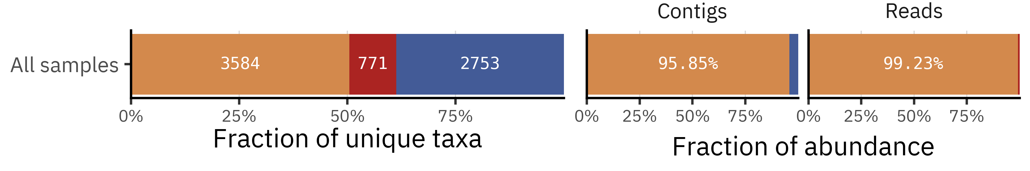

If we pool all 21 samples and look at the union of taxa detected by each method, the picture becomes more puzzling. The single bar for “All samples” shows that around half of all taxa are shared (3584), but among the remaining half many more taxa are unique to contigs (2753) than to reads (771). At first sight this seems to contradict the per-sample view, where reads tend to have more unique taxa than contigs.

This apparent paradox comes from the fact that the union treats each taxon only once, regardless of how many samples it appears in. A taxon that is unique to contigs and occurs in only one sample counts exactly as much as a taxon that is unique to reads but recurs across many samples. To understand whether contig-only taxa are truly widespread or mostly single-sample curiosities, we now look at the prevalence of each taxon across samples and compare how often taxa that are unique to each pipeline are actually observed.

Prevalence code

df = df_wide_rel.copy()

# Presence / absence per sample
presence = (df > 0).groupby(level="kind").sum()

reads_prev = presence.loc["reads"]
contigs_prev = presence.loc["contigs"]

# Global unique sets
reads_only_mask = (reads_prev > 0) & (contigs_prev == 0)
contigs_only_mask = (contigs_prev > 0) & (reads_prev == 0)

reads_only_taxa = reads_prev[reads_only_mask]
contigs_only_taxa = contigs_prev[contigs_only_mask]

# Long table: one row per taxid with its prevalence and group
prev_long = pd.concat(
    [
        pd.DataFrame(
            {
                "taxid": reads_only_taxa.index.astype(str),
                "prevalence": reads_only_taxa.values,
                "group": "Reads only",
            }
        ),
        pd.DataFrame(
            {
                "taxid": contigs_only_taxa.index.astype(str),
                "prevalence": contigs_only_taxa.values,
                "group": "Contigs only",
            }
        ),
    ],
    ignore_index=True,
)

# Aggregate to counts per prevalence
prev_counts = (
    prev_long.groupby(["group", "prevalence"]).size().reset_index(name="n_taxa")
)

# Optional sanity check of singleton fractions
reads_singletons = prev_counts.query("group == 'Reads only' & prevalence == 1")[
    "n_taxa"
].iloc[0]
reads_total = prev_counts.query("group == 'Reads only'")["n_taxa"].sum()
contigs_singletons = prev_counts.query("group == 'Contigs only' & prevalence == 1")[
    "n_taxa"
].iloc[0]
contigs_total = prev_counts.query("group == 'Contigs only'")["n_taxa"].sum()

print(
    "Reads only:   %d / %d taxa are singletons (%.1f%%)"
    % (reads_singletons, reads_total, 100 * reads_singletons / reads_total)
)
print(
    "Contigs only: %d / %d taxa are singletons (%.1f%%)"
    % (contigs_singletons, contigs_total, 100 * contigs_singletons / contigs_total)
)

Reads only:   457 / 771 taxa are singletons (59.3%)
Contigs only: 2276 / 2753 taxa are singletons (82.7%)

Log Scale
Normal scale

Show Code

p_prev = (
    p9.ggplot(prev_counts, p9.aes("prevalence", "n_taxa", fill="group"))
    + p9.geom_col(position=p9.position_dodge2(preserve="single"))
    + p9.scale_x_continuous(breaks=range(1, int(prev_counts["prevalence"].max()) + 1))
    # log scale helps, because prevalence=1 dominates
    + p9.scale_y_continuous(trans="log10")
    + p9.labs(
        x="Number of samples where taxon is detected",
        y="Number of taxa (log scale)",
        fill="",
        title="Prevalence of taxa that are unique to each pipeline",
    )
    + p9.theme(
        figure_size=(6, 4),
        legend_position="top",
    )
)

p_prev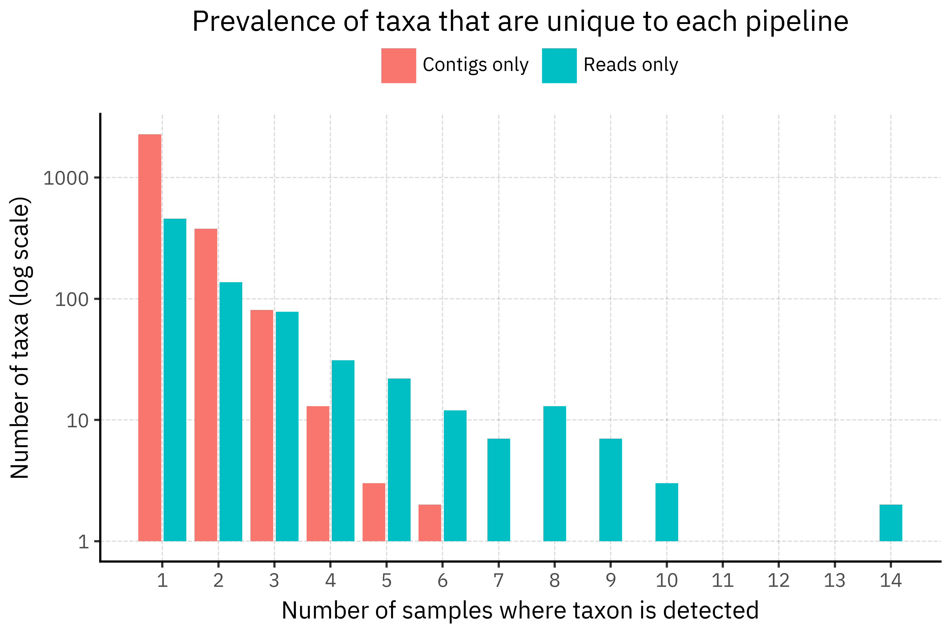

Show Code

p_prev = (
    p9.ggplot(prev_counts, p9.aes("prevalence", "n_taxa", fill="group"))
    + p9.geom_col(position=p9.position_dodge2(preserve="single"))
    + p9.scale_x_continuous(breaks=range(1, int(prev_counts["prevalence"].max()) + 1))
    + p9.labs(
        x="Number of samples where taxon is detected",
        y="Number of taxa",
        fill="",
        title="Prevalence of taxa that are unique to each pipeline",
    )
    + p9.theme(
        figure_size=(6, 4),
        legend_position="top",
    )
)
p_prev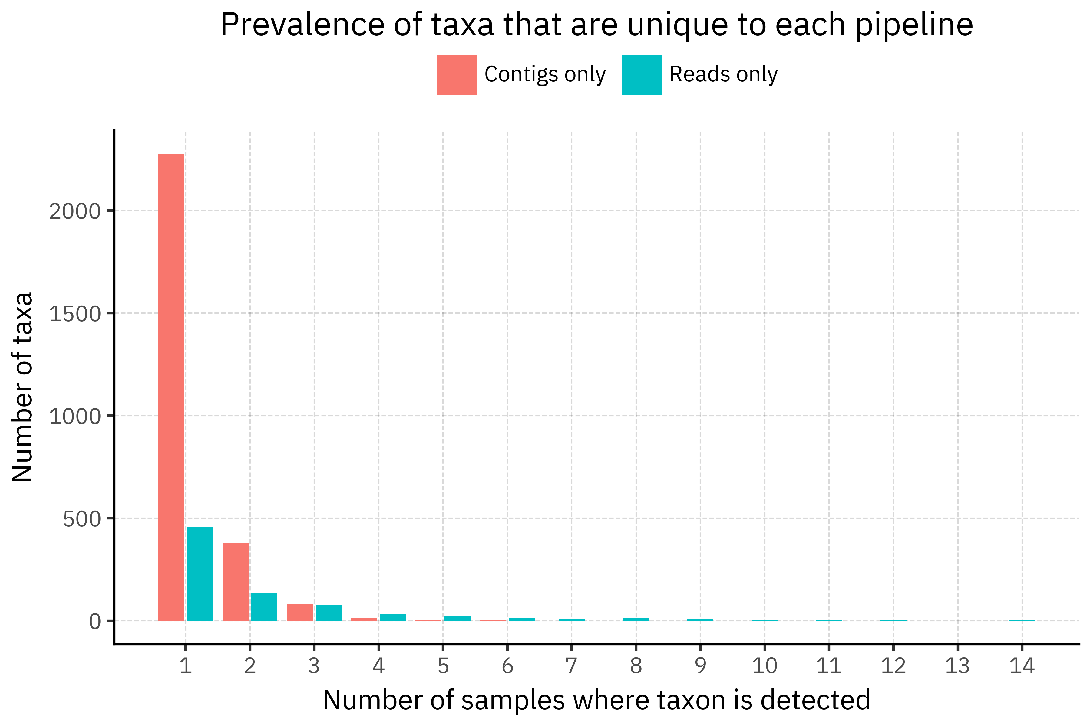

The prevalence plot shows that the paradox is mostly a union-of-singletons effect. Among taxa that are unique to each pipeline, contigs-only taxa are overwhelmingly singletons (82.7 % appear in just one sample), while reads-only taxa have a much heavier tail and are more often seen in several samples. So when we take the union across all samples, each assembly contributes its own small cloud of contig-only taxa that never reappear, inflating the contigs-only count, whereas reads-only taxa are reused across samples and do not grow as fast.

A plausible explanation is that assemblies are more sensitive to slight differences in coverage and assembly graph resolution. With ultra-low biomass and amplification noise, each sample can produce slightly different contigs that happen to hit different reference genomes or strains in DIAMOND+MEGAN, generating many sample-specific taxids in the long tail. Direct read classification, although noisier at the individual read level, tends to scatter ambiguous hits across a smaller set of higher level nodes, which then recur in multiple samples. In other words, assemblies introduce more idiosyncratic rare taxa, while reads produce a more stable but still low-abundance tail?

The next step is to see how robust these patterns are when we collapse the data to broader taxonomic ranks (species, genus, family), which reduces artificial differences caused by one pipeline assigning to strains while the other stays at higher levels.

Looking at the taxa

Since we have the taxids of each taxa, we can use the NCBI Taxonomy database to get the full lineage of each taxa.

I am going to use ete3 to do this and write a simple auxiliary function to get (1) the rank of each taxa and (2) the name of the taxa:

ncbi = NCBITaxa()


def annotate_taxids(taxids, ncbi: NCBITaxa) -> pd.DataFrame:
    """
    Return a DataFrame with one row per taxid and its NCBI rank and name.
    Missing ranks/names are set to None.
    """
    # make sure taxids are unique, but preserve order
    taxids = list(dict.fromkeys(int(t) for t in taxids))

    rank_dict = ncbi.get_rank(taxids)  # {taxid: rank}
    name_dict = ncbi.get_taxid_translator(taxids)  # {taxid: name}

    rows = []
    for tid in taxids:
        rows.append(
            {
                "taxid": tid,
                "rank": rank_dict.get(tid),  # None if missing
                "name": name_dict.get(tid),
            }
        )

    return pd.DataFrame(rows)

Let’s first take a look at the taxa that we saw were quite prevalent (over 8 samples) yet only appeared in reads but not in assemblies:

Show Code

annotated_prev = annotate_taxids(
    prev_long.query("prevalence > 8").taxid, ncbi=ncbi
).assign(taxid=lambda x: x.taxid.astype(str))
annotated_prev.merge(prev_long, on="taxid", how="inner").sort_values(
    "prevalence", ascending=False
).set_index("taxid")

	rank	name	prevalence	group
taxid
3869	genus	Lupinus	14	Reads only
227292	no rank	Sinorhizobium/Ensifer group	14	Reads only
2604474	no rank	unclassified Mortierella	12	Reads only
2233855	clade	indigoferoid/millettioid clade	11	Reads only
41087	infraorder	Elateriformia	10	Reads only
203491	order	Fusobacteriales	10	Reads only
2052145	no rank	unclassified Blastocatellia	10	Reads only
36086	genus	Trichuris	9	Reads only
77643	species group	Mycobacterium tuberculosis complex	9	Reads only
134549	class	Spartobacteria	9	Reads only
213115	order	Desulfovibrionales	9	Reads only
539002	no rank	Bacillales incertae sedis	9	Reads only
2685293	no rank	unclassified Subdoligranulum	9	Reads only
2892396	genus	Vescimonas	9	Reads only

So, as we can see, the most prevalent taxa which is present in one pipeline but doesn’t show up in the other one is the genus Lupinus, a genus of flowering plants in the pea family.

It is present in 14 different read samples but not in any of the assemblies. Now, that is rather weird, but might we be just conflating different depths of identification into uniqueness?

Let’s generate a series of helper functions to translate taxids into full taxonomic lineages, extract the relevant ranks, and get the information at the levels we are interested in.

RELEVANT_RANKS = [
    "domain",
    "kingdom",
    "phylum",
    "class",
    "order",
    "family",
    "genus",
    "species",
]

def get_relevant_ranks_taxids(taxid: int, ncbi: NCBITaxa) -> dict:
    lineage = ncbi.get_lineage(taxid)  # list of taxids in order
    ranks = ncbi.get_rank(lineage)  # {taxid: rank_name}

    result = {}
    for rank in RELEVANT_RANKS:
        for tid in lineage:
            if ranks.get(tid) == rank:
                result[rank] = tid
                break  # only take the first match in lineage

    return result


def get_relevant_rank_names(taxid: int, ncbi: NCBITaxa) -> dict:
    """
    Return {rank_name: taxon_name} for the ranks in RELEVANT_RANKS
    present in the lineage of `taxid`.
    """
    rank_taxids = get_relevant_ranks_taxids(taxid, ncbi)  # {rank: taxid}
    taxids = list(rank_taxids.values())

    if not taxids:
        return {}

    names = ncbi.get_taxid_translator(taxids)  # {taxid: name}

    rank_names = {rank: names[tid] for rank, tid in rank_taxids.items() if tid in names}
    return rank_names


def get_relevant_ranks_with_names(taxid: int, ncbi: NCBITaxa) -> dict:
    rank_taxids = get_relevant_ranks_taxids(taxid, ncbi)
    taxids = list(rank_taxids.values())
    names = ncbi.get_taxid_translator(taxids) if taxids else {}
    return {
        rank: {"taxid": tid, "name": names.get(tid)}
        for rank, tid in rank_taxids.items()
    }


def annotate_taxids_with_ranks(taxids, ncbi: NCBITaxa) -> pd.DataFrame:
    """
    Given an iterable of taxids, return a DataFrame with:
      - one row per original taxid
      - columns: 'taxid', plus '<rank>_taxid' and '<rank>_name'
        for each rank in RELEVANT_RANKS.
    """
    records = []
    for t in taxids:
        t_int = int(t)
        info = get_relevant_ranks_with_names(t_int, ncbi)

        row = {"taxid": t_int}
        for rank in RELEVANT_RANKS:
            if rank in info:
                row[f"{rank}"] = info[rank]["name"]
            else:
                row[f"{rank}"] = None

        records.append(row)

    return pd.DataFrame(records)

Now, if we annotate the three sets of taxids:

only_contigs_tax_df = annotate_taxids_with_ranks(only_contigs, ncbi=ncbi)
only_reads_tax_df = annotate_taxids_with_ranks(only_reads, ncbi=ncbi)
shared_tax_df = annotate_taxids_with_ranks(shared, ncbi=ncbi)
all_tax_df = annotate_taxids_with_ranks(union, ncbi=ncbi)

And look for taxids matching genus Lupinus in all three:

only_reads_tax_df.query('genus=="Lupinus"')

	taxid	domain	kingdom	phylum	class	order	family	genus	species
703	3869	Eukaryota	Viridiplantae	Streptophyta	Magnoliopsida	Fabales	Fabaceae	Lupinus	None

only_contigs_tax_df.query('genus=="Lupinus"')

	taxid	domain	kingdom	phylum	class	order	family	genus	species
1350	3871	Eukaryota	Viridiplantae	Streptophyta	Magnoliopsida	Fabales	Fabaceae	Lupinus	Lupinus angustifolius

shared_tax_df.query('genus=="Lupinus"')

	taxid	domain	kingdom	phylum	class	order	family	genus	species
1757	3870	Eukaryota	Viridiplantae	Streptophyta	Magnoliopsida	Fabales	Fabaceae	Lupinus	Lupinus albus

all_tax_df.query('genus=="Lupinus"')

	taxid	domain	kingdom	phylum	class	order	family	genus	species
1211	3869	Eukaryota	Viridiplantae	Streptophyta	Magnoliopsida	Fabales	Fabaceae	Lupinus	None
1212	3870	Eukaryota	Viridiplantae	Streptophyta	Magnoliopsida	Fabales	Fabaceae	Lupinus	Lupinus albus
1213	3871	Eukaryota	Viridiplantae	Streptophyta	Magnoliopsida	Fabales	Fabaceae	Lupinus	Lupinus angustifolius

df_wide_rel[[3869, 3870, 3871]].map(lambda x: x > 0).groupby("kind").sum()

taxid	3869	3870	3871
kind
contigs	0	20	3
reads	14	21	0

At the raw taxid level, taxid 3869 (generic Lupinus) is detected in 14 read samples but never in contigs, so it appears as one of the most prevalent reads-only taxa. However, contigs frequently classify the same signal as Lupinus albus (taxid 3870) or another Lupinus species (taxid 3871). When we collapse to the genus level, all three taxids merge into a single Lupinus node that is clearly shared between methods.

This shows that much of the apparent disagreement at taxid level comes from differences in depth of classification rather than true presence or absence of a genus.

Species and Genus-level analysis

In the previous section (Lupinus example), we saw that some “reads-only” vs “contigs-only” differences at the raw taxid level are actually rank-depth effects: the same genus may be present in both pipelines, but one pipeline stops higher in the taxonomy more often.

To make that explicit, let’s first quantify how much of each sample’s relative abundance can be assigned at progressively deeper ranks (Domain → Species), and then inspect the most abundant taxa at species and genus level side-by-side for each sample.

For each rank r, I compute:

ra_r = sum(relative_abundance) over taxa where rank r is not null (within each sample_id × kind).

This gives a simple “assignment depth” curve: if a pipeline often stops at Family/Genus, the Species bar will necessarily be smaller, even if the high-rank structure is similar.

Identification depth computation

long_assigned_df = (
    df_wide_rel.reset_index()
    .melt(
        id_vars=["sample_id", "kind"], var_name="taxid", value_name="relative_abundance"
    )
    .merge(all_tax_df, on="taxid", how="left")
    .replace({None: pd.NA})
)

depth_per_sample_df = (
    pl.from_pandas(long_assigned_df)
    .lazy()
    .group_by(["sample_id", "kind"])
    .agg(
        # abundance "assigned" at each rank = sum(relative_abundance where rank is not null)
        *[
            pl.col("relative_abundance")
            .filter(pl.col(r).is_not_null())
            .sum()
            .alias(f"ra_{r}")
            for r in RELEVANT_RANKS
        ],
    )
    .collect()
)

depth_all_df = (
    depth_per_sample_df.lazy()
    .group_by("kind")
    .agg(
        *[pl.col(f"ra_{r}").mean() for r in RELEVANT_RANKS],
        *[pl.col(f"ra_{r}").std().alias(f"std_{r}") for r in RELEVANT_RANKS],
        *[pl.col(f"ra_{r}").min().alias(f"min_{r}") for r in RELEVANT_RANKS],
        *[pl.col(f"ra_{r}").max().alias(f"max_{r}") for r in RELEVANT_RANKS],
        *[pl.col(f"ra_{r}").quantile(0.25).alias(f"q25_{r}") for r in RELEVANT_RANKS],
        *[pl.col(f"ra_{r}").quantile(0.75).alias(f"q75_{r}") for r in RELEVANT_RANKS],
        *[pl.col(f"ra_{r}").quantile(0.95).alias(f"q95_{r}") for r in RELEVANT_RANKS],
        *[pl.col(f"ra_{r}").quantile(0.05).alias(f"q05_{r}") for r in RELEVANT_RANKS],
    )
    .with_columns(
        pl.col("kind").replace({"contigs": "Contigs", "reads": "HiFi reads"}),
    )
    .collect()
)

Show Code

labels = list(map(lambda x: x.capitalize(), RELEVANT_RANKS[::-1]))
(
    depth_all_df.unpivot(index=["kind"])
    .with_columns(
        pl.col("variable").str.split("_").list.get(1).alias("rank"),
        pl.col("variable").str.split("_").list.get(0).alias("metric"),
    )
    .drop("variable")
    .filter(pl.col("metric").is_in(["ra", "std"]))
    .pivot(index=["rank", "kind"], on="metric", values="value")
    .pipe(
        lambda dd: p9.ggplot(dd)
        + p9.aes("rank.str.capitalize()", "ra", fill="kind", group="kind")
        + p9.geom_errorbar(
            p9.aes(ymax="ra + std", ymin="ra - std", color="kind"),
            position=p9.position_dodge(preserve="single", width=0.775),
            width=0.3,
        )
        + p9.geom_col(
            position=p9.position_dodge(preserve="single", width=0.825), width=0.8
        )
        + p9.scale_x_discrete(limits=labels)
        + p9.scale_y_continuous(expand=(0, 0), limits=(0, 1.1), labels=percent_format())
        + p9.coord_flip()
        + p9.labs(
            x="",
            y="Percentage of all assigned reads",
            fill="",
            color="",
            title="Rate of identification",
        )
        + p9.theme(figure_size=(4, 3), axis_title=p9.element_text(size=10))
    )
)

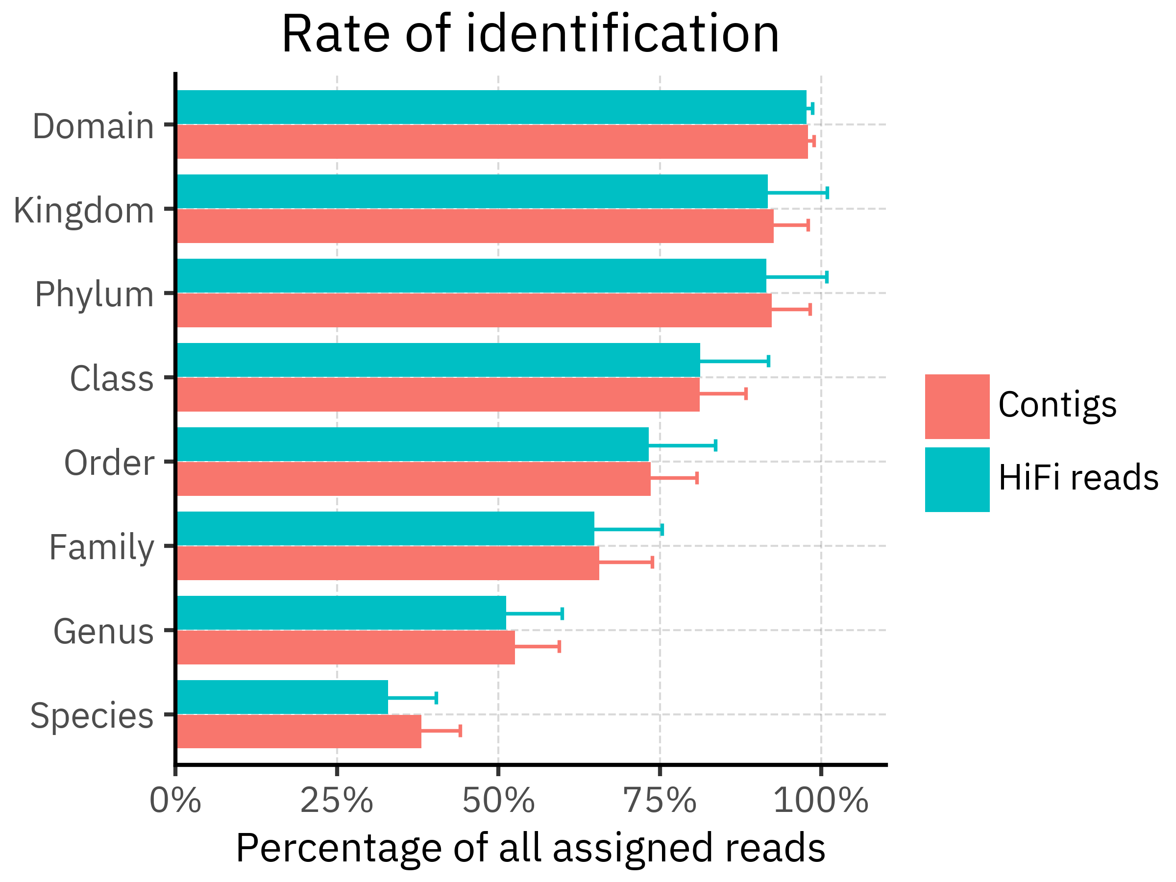
In our data, both pipelines assign almost all abundance at Domain/Kingdom/Phylum, but the assigned fraction drops steadily towards Genus and Species. Contigs are slightly higher at most ranks, but specially at the Genus and Species levels, consistent with contigs providing more specific placements for part of the community. The differences, however, are not really strong in either case.

Note: this figure summarizes relative abundance within each profile, so it should be interpreted as “fraction of assigned signal” rather than a statement about absolute read counts.

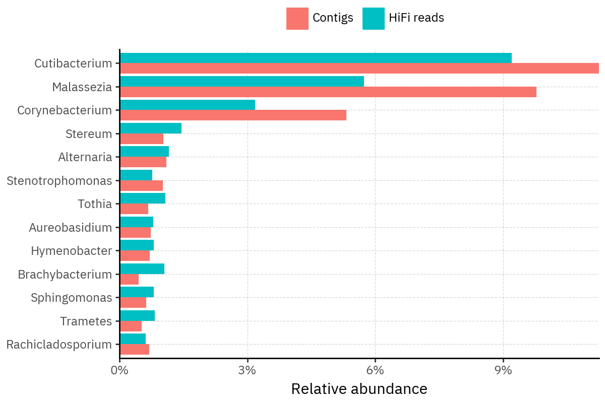
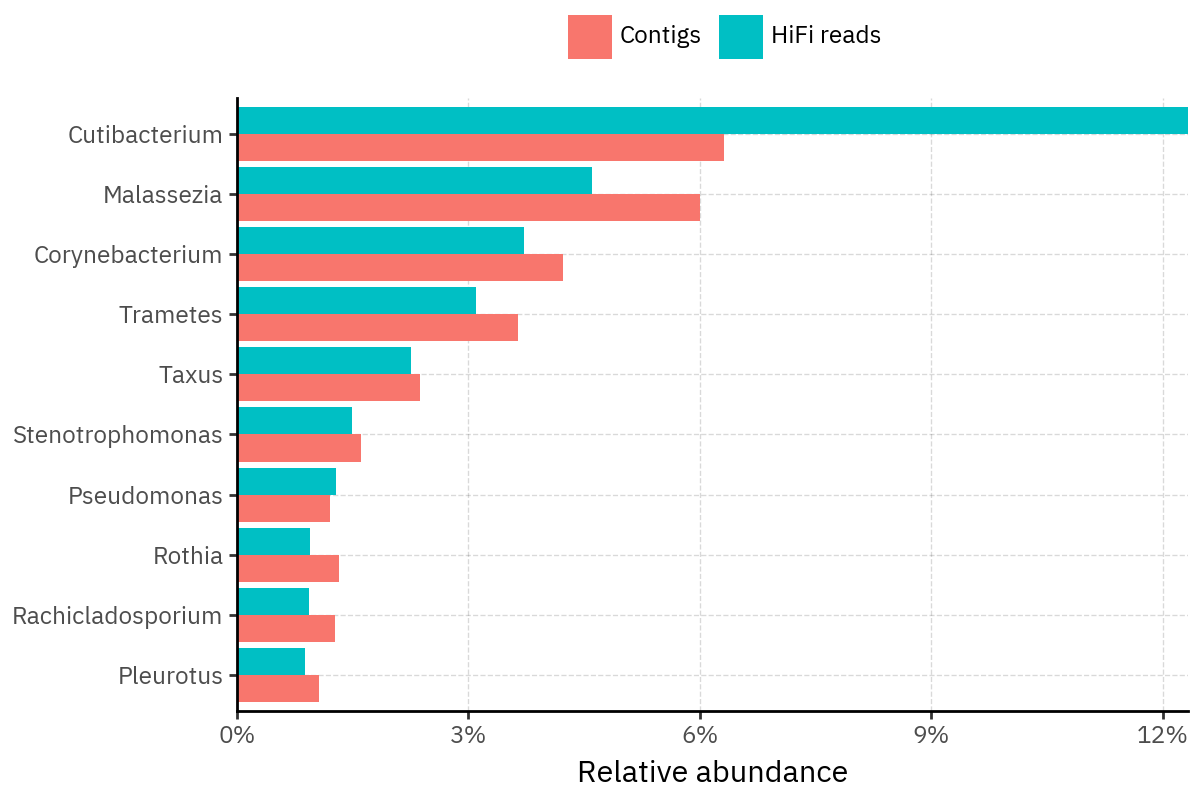
Top 10 species by sample:

To understand what drives the differences at the deepest rank, I plot the Top-10 species per sample for each pipeline. For each sample, the y-axis includes the union of taxa that appear in the top-10 of either method, so some panels can show more than 10 rows.

Show Code

OUT_DIR = Path("_generated/top10_tabs")
FIG_DIR = OUT_DIR / "figs"
FIG_DIR.mkdir(parents=True, exist_ok=True)


def slug(s: str) -> str:
    return re.sub(r"[^A-Za-z0-9_.-]+", "_", str(s))


species_ra_df = (
    pl.from_pandas(long_assigned_df)
    .lazy()
    .filter(pl.col("relative_abundance") > 0)
    .filter(pl.col("species") != "Unassigned")
    .with_columns([pl.col(c).fill_null("Unassigned") for c in RELEVANT_RANKS])
    .group_by(["sample_id", "kind"] + RELEVANT_RANKS)
    .agg(pl.col("relative_abundance").sum().alias("ra"))
    .sort(["sample_id", "kind", "ra"], descending=[False, False, True])
    .collect()
)

top10_species_per_sample = species_ra_df.group_by(["sample_id", "kind"]).head(10)

samples = (
    top10_species_per_sample.select("sample_id")
    .unique()
    .sort("sample_id")
    .to_series()
    .to_list()
)

lines = []
lines.append(
    "::: {.panel-tabset}\n\n"
)  # fenced div, more robust than heading-attribute tabset

for s in samples:
    s_slug = slug(s)

    curr_top10 = (
        top10_species_per_sample.filter(pl.col("sample_id") == s)
        .get_column("species")
        .to_list()
    )

    dd = (
        species_ra_df.with_columns(
            pl.col("kind").replace({"contigs": "Contigs", "reads": "HiFi reads"})
        )
        .filter(pl.col("sample_id") == s)
        .filter(pl.col("species").is_in(curr_top10))
    )

    p = (
        p9.ggplot(dd)
        + p9.aes("reorder(species, ra)", "ra", fill="kind")
        + p9.geom_col(position=p9.position_dodge(preserve="single"))
        + p9.coord_flip()
        + p9.scale_y_continuous(labels=percent_format(), expand=(0, 0))
        + p9.labs(x="", y="Relative abundance", fill="")
        + p9.theme(legend_position="top", figure_size=(6, 4))
    )

    fig_path = FIG_DIR / f"top10_species_{s_slug}.png"
    p.save(fig_path, dpi=200, verbose=False)

    # Important: no leading spaces on headings
    lines.append(f"### {s}\n\n")
    lines.append(f"![]({fig_path.as_posix()})\n\n")

lines.append(":::\n")

md_path = OUT_DIR / "top10_tabs.md"
md_path.write_text("".join(lines), encoding="utf-8")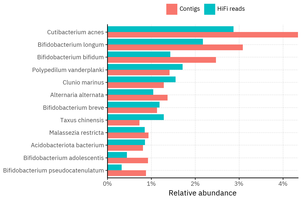

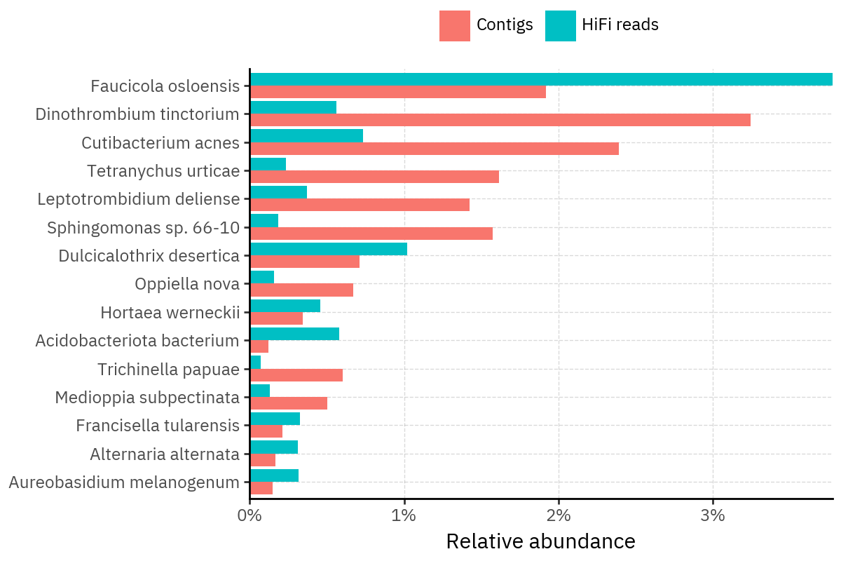
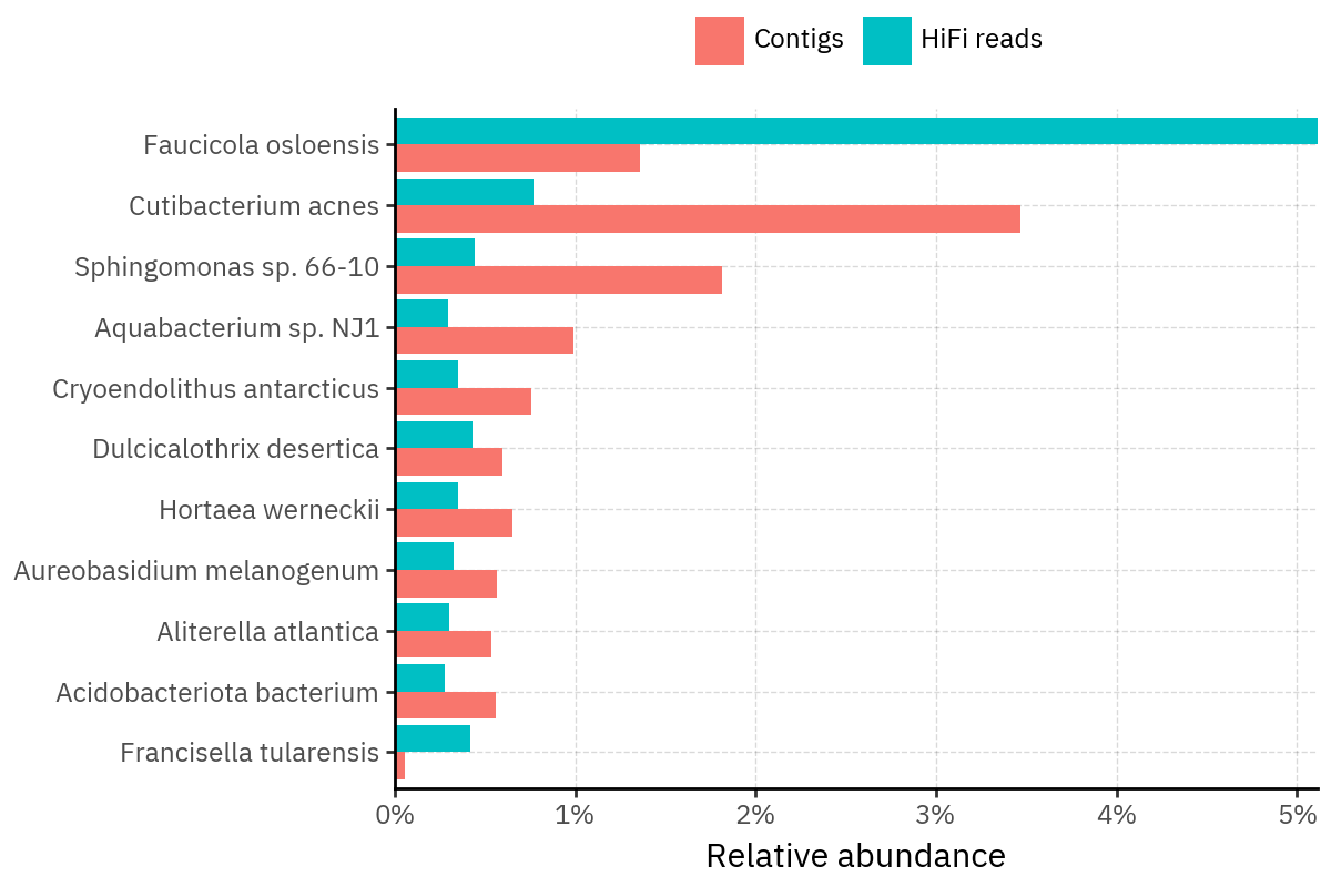
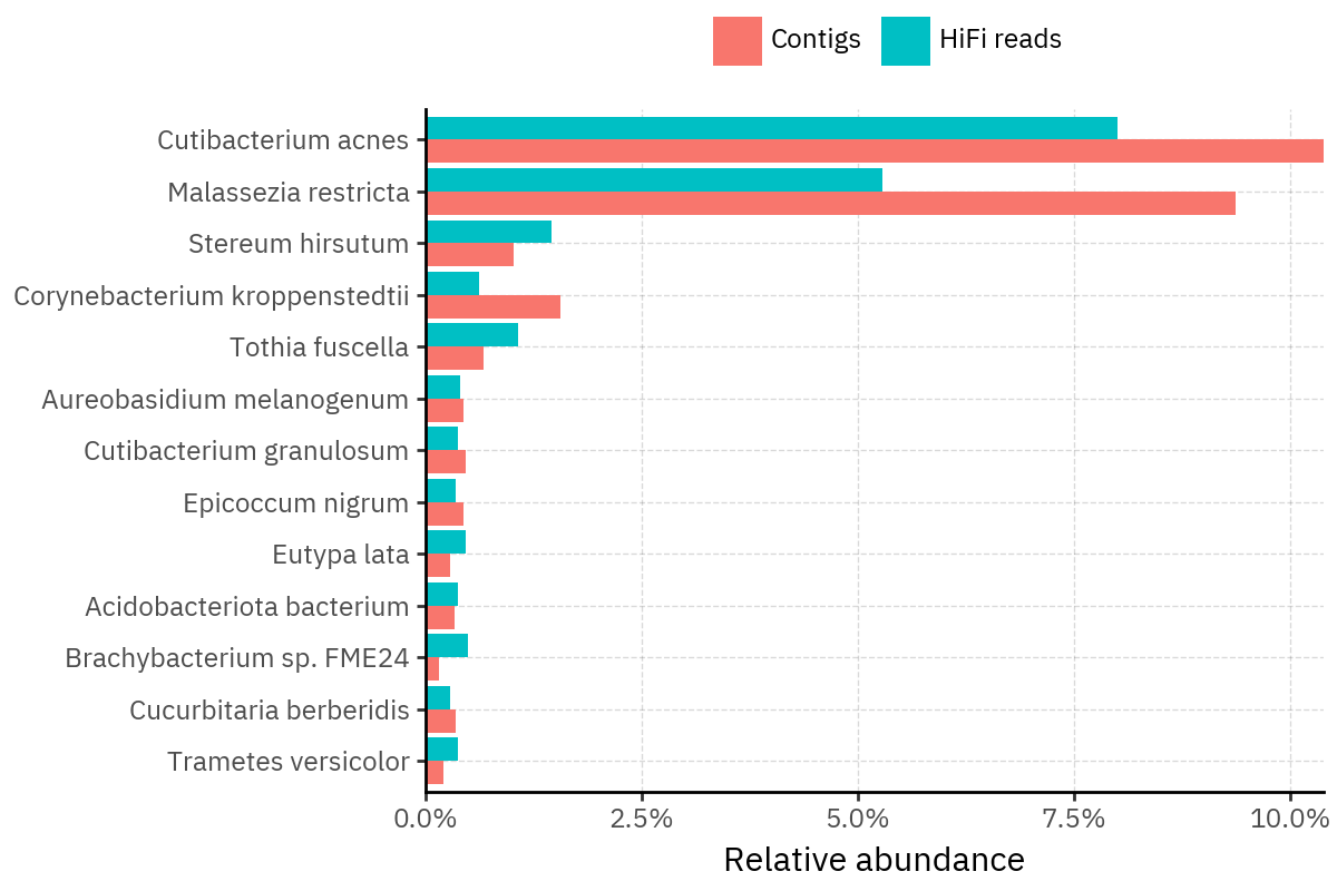
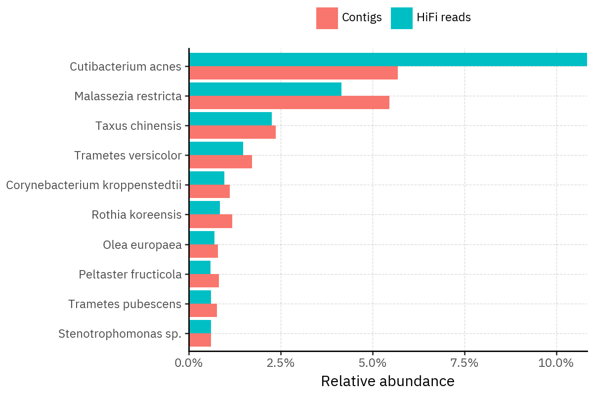
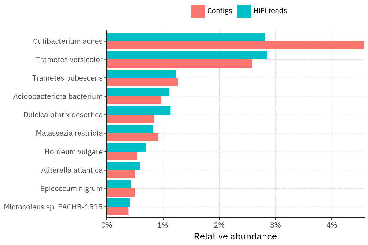
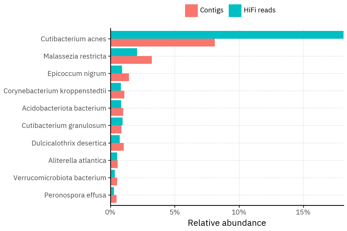
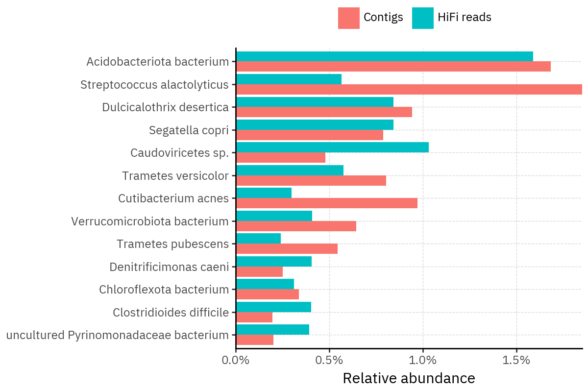
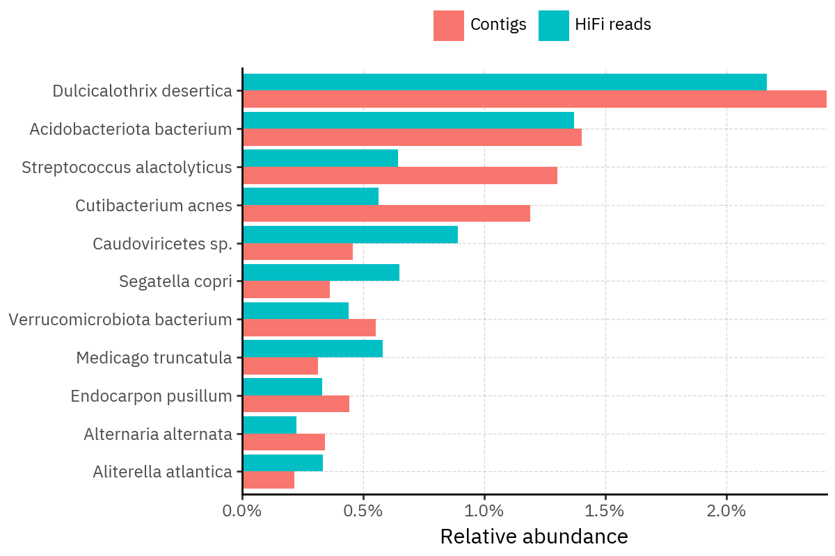
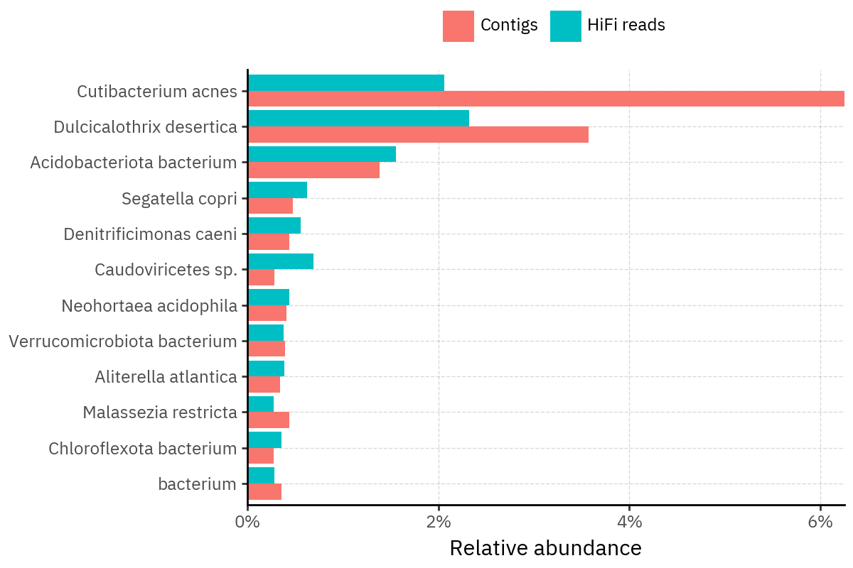
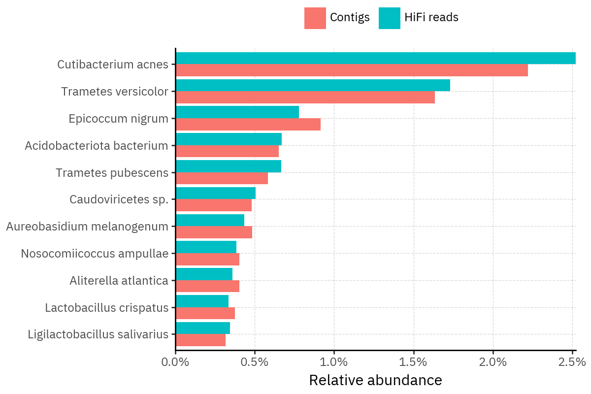
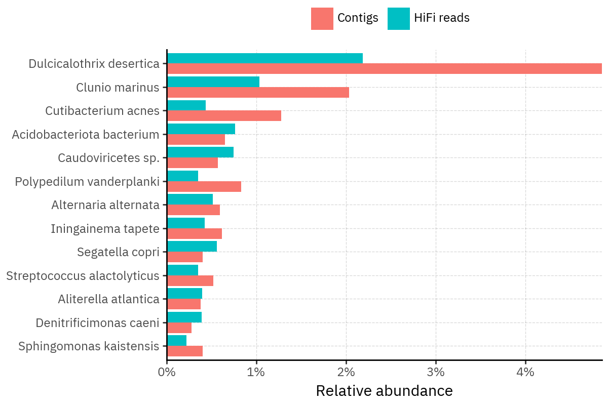
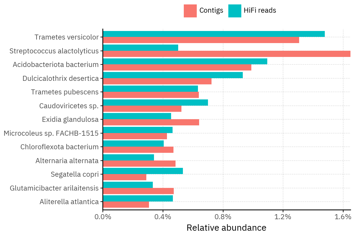
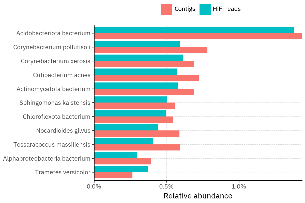
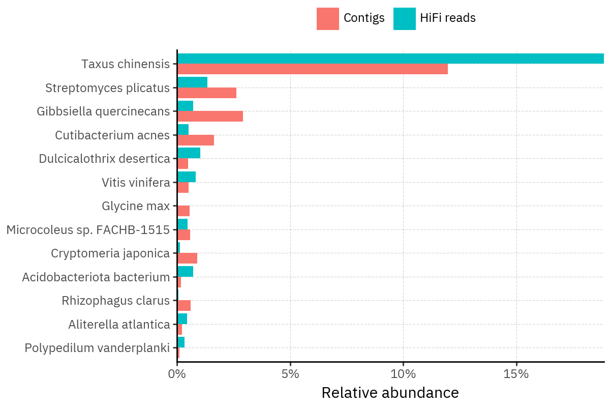
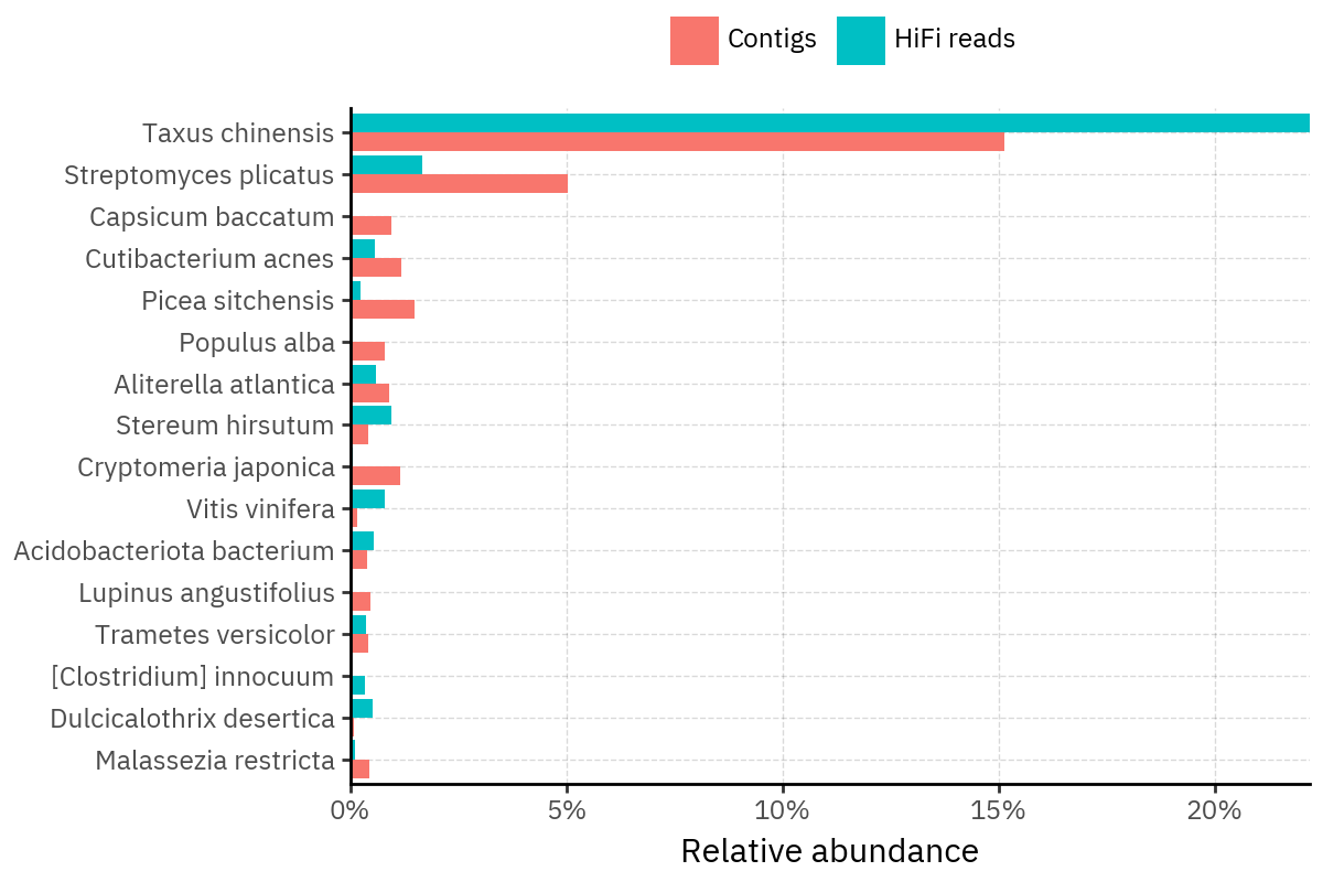
Across samples, the “headline” taxa are often shared, but their estimated relative abundances can shift between reads and contigs. For example, in KS001 and KS045, Cutibacterium acnes is detected in both pipelines but appears substantially higher in contigs, while several other taxa show smaller method-specific shifts.

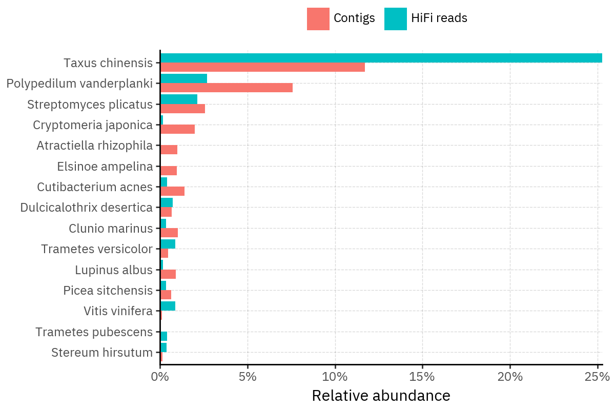
Some samples show a very strong dominant taxon that both methods recover, but with different magnitude. For instance, KS112 is dominated by Taxus chinensis in both pipelines, with reads reporting a much larger fraction than contigs.

Overall, these panels suggest that many differences are not “new biology” appearing in one pipeline only, but a combination of (i) deeper vs shallower placement, and (ii) reweighting of the top taxa when collapsing evidence into contigs.

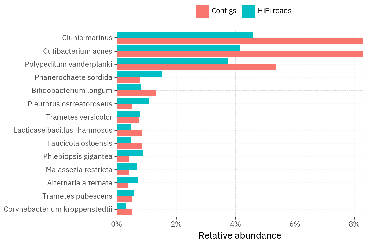
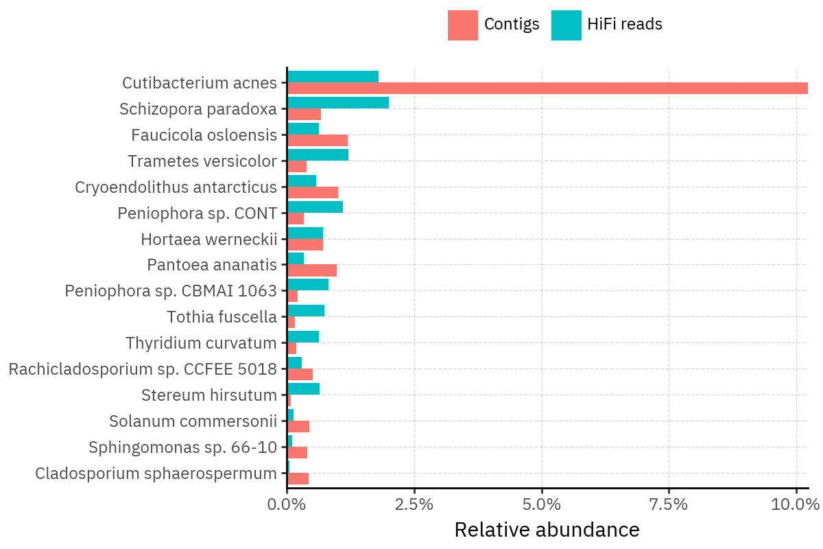
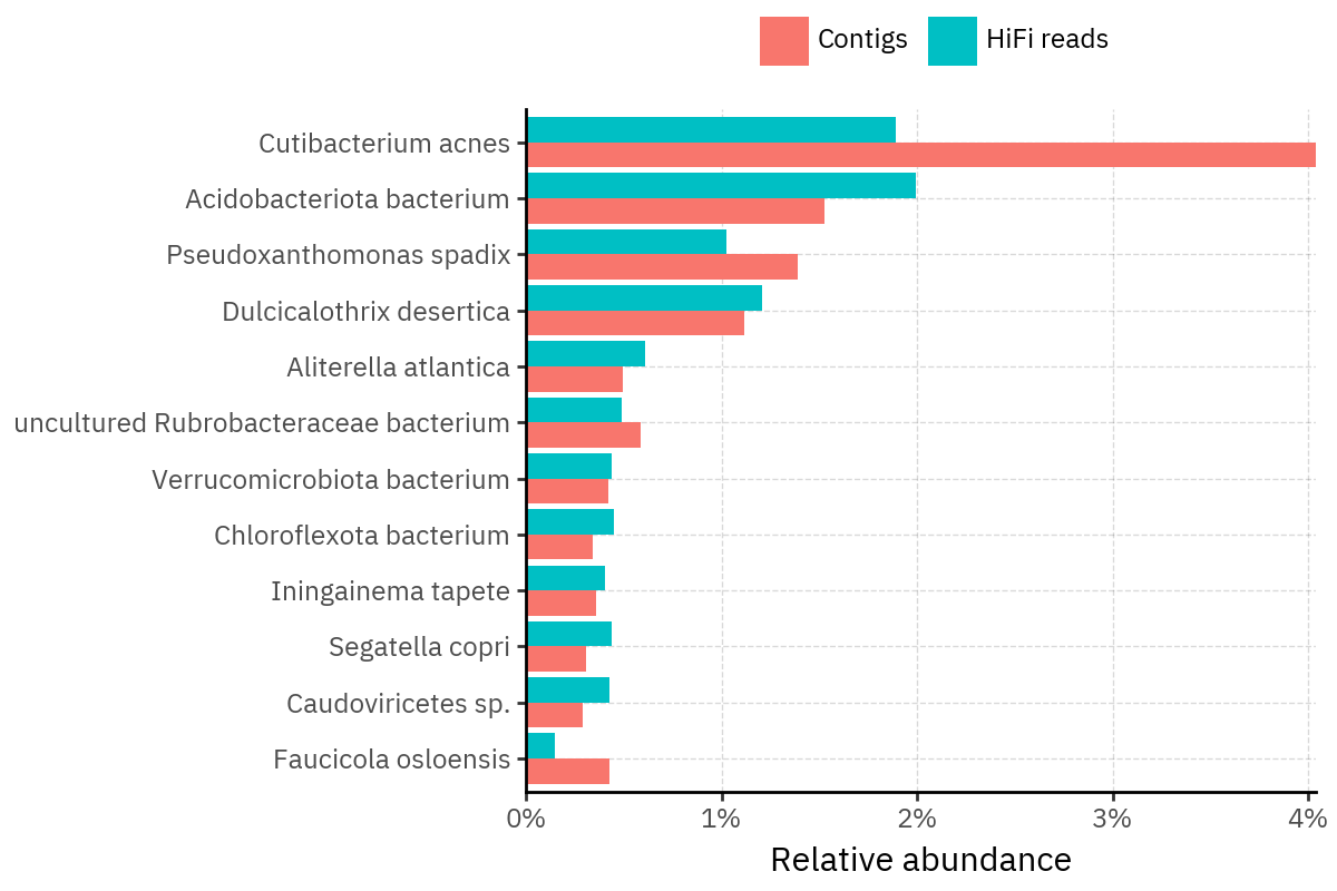
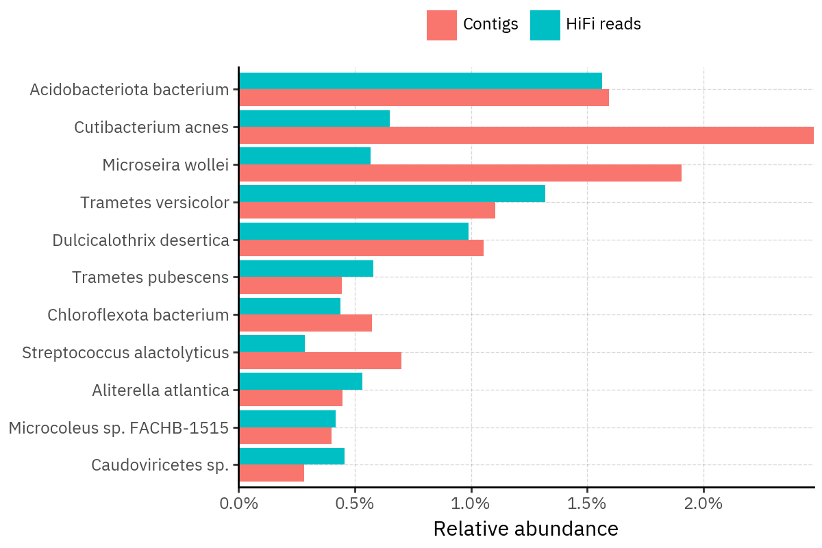
Top 10 Genus per sample

Show Code

OUT_DIR = Path("_generated/top10_tabs_g")
FIG_DIR = OUT_DIR / "figs/genera"
FIG_DIR.mkdir(parents=True, exist_ok=True)


def slug(s: str) -> str:
    return re.sub(r"[^A-Za-z0-9_.-]+", "_", str(s))


genus_ra_df = (
    pl.from_pandas(long_assigned_df)
    .lazy()
    .filter(pl.col("relative_abundance") > 0)
    .filter(pl.col("genus") != "Unassigned")
    .with_columns([pl.col(c).fill_null("Unassigned") for c in RELEVANT_RANKS])
    .group_by(["sample_id", "kind"] + RELEVANT_RANKS[:-1])
    .agg(pl.col("relative_abundance").sum().alias("ra"))
    .sort(["sample_id", "kind", "ra"], descending=[False, False, True])
    .collect()
)

top10_genus_per_sample = genus_ra_df.group_by(["sample_id", "kind"]).head(10)

samples = (
    top10_genus_per_sample.select("sample_id")
    .unique()
    .sort("sample_id")
    .to_series()
    .to_list()
)

lines = []
lines.append(
    "::: {.panel-tabset}\n\n"
)  # fenced div, more robust than heading-attribute tabset

for s in samples:
    s_slug = slug(s)

    curr_top10 = (
        top10_genus_per_sample.filter(pl.col("sample_id") == s)
        .get_column("genus")
        .to_list()
    )

    dd = (
        genus_ra_df.with_columns(
            pl.col("kind").replace({"contigs": "Contigs", "reads": "HiFi reads"})
        )
        .filter(pl.col("sample_id") == s)
        .filter(pl.col("genus").is_in(curr_top10))
    )

    p = (
        p9.ggplot(dd)
        + p9.aes("reorder(genus, ra)", "ra", fill="kind")
        + p9.geom_col(position=p9.position_dodge(preserve="single"))
        + p9.coord_flip()
        + p9.scale_y_continuous(labels=percent_format(), expand=(0, 0))
        + p9.labs(x="", y="Relative abundance", fill="")
        + p9.theme(legend_position="top", figure_size=(6, 4))
    )

    fig_path = FIG_DIR / f"top10_genus_{s_slug}.png"
    p.save(fig_path, dpi=200, verbose=False)

    # Important: no leading spaces on headings
    lines.append(f"### {s}\n\n")
    lines.append(f"![]({fig_path.as_posix()})\n\n")

lines.append(":::\n")

md_path = OUT_DIR / "top10_tabs.md"
md_path.write_text("".join(lines), encoding="utf-8")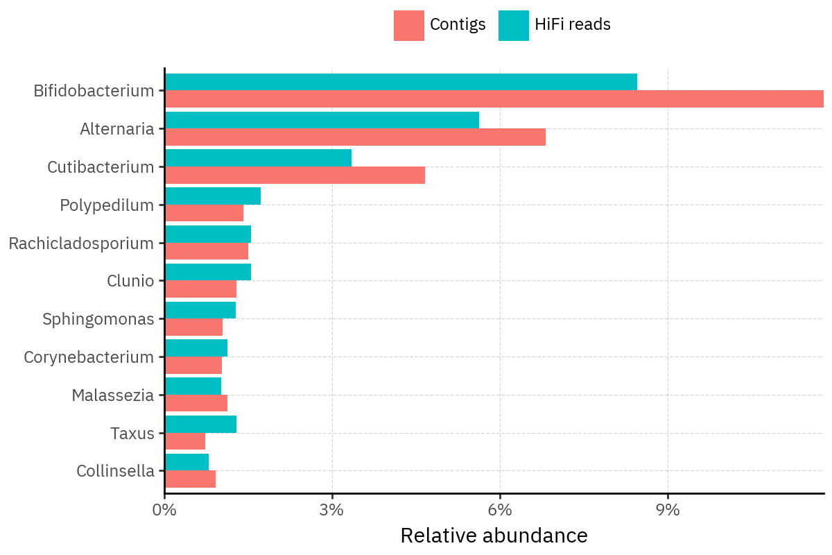

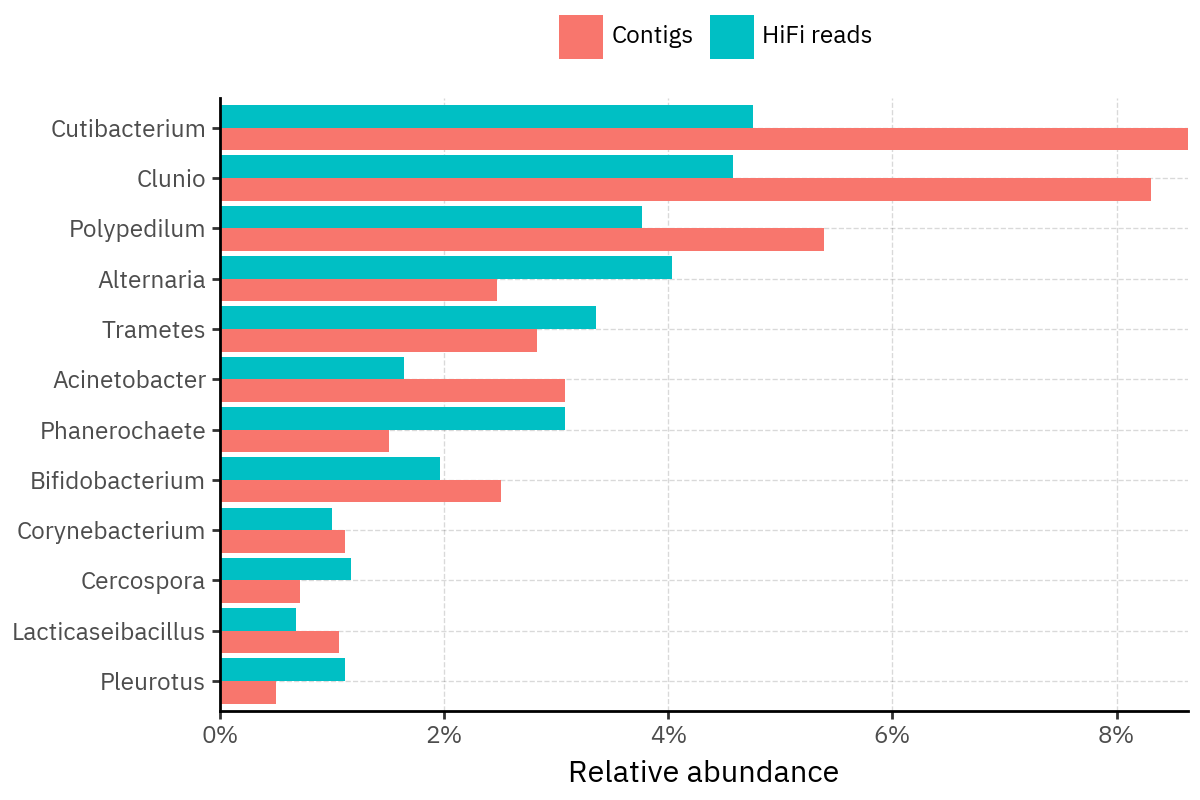
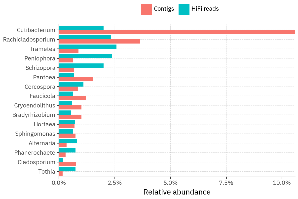
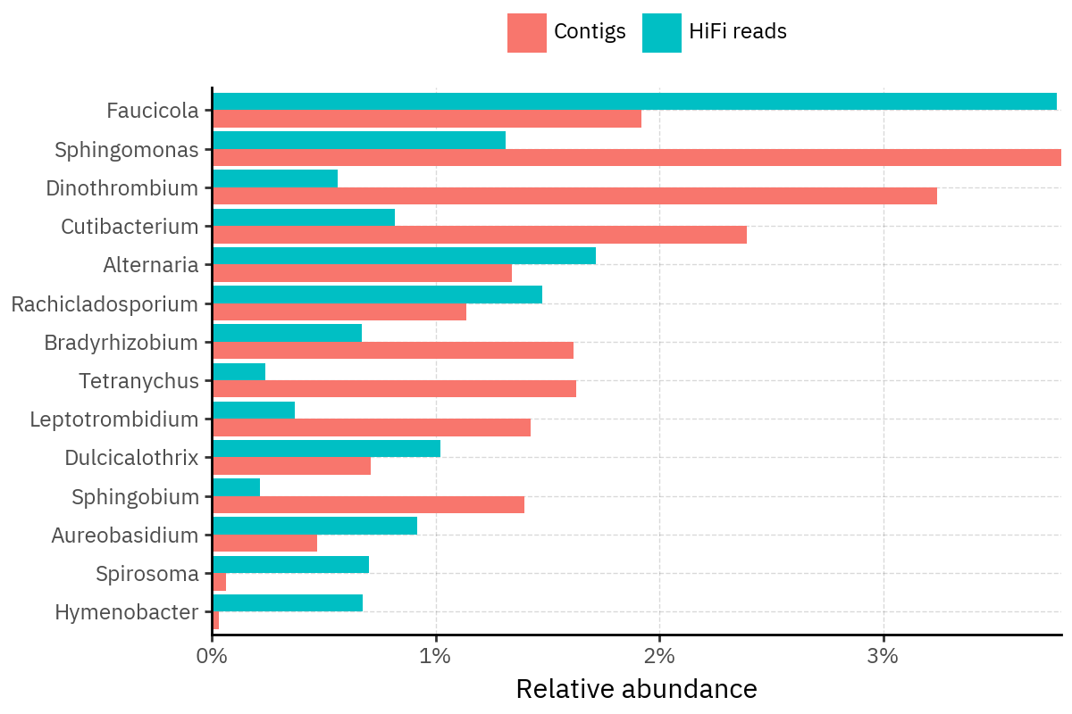
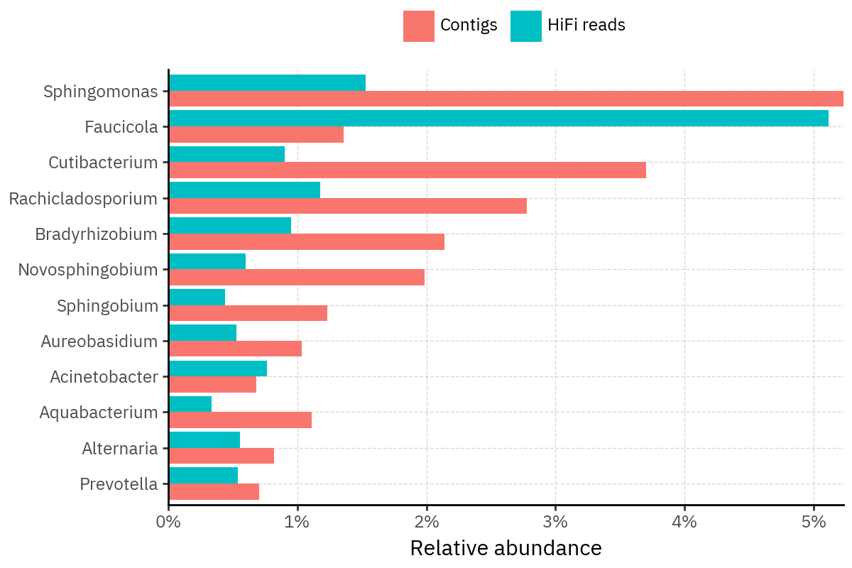
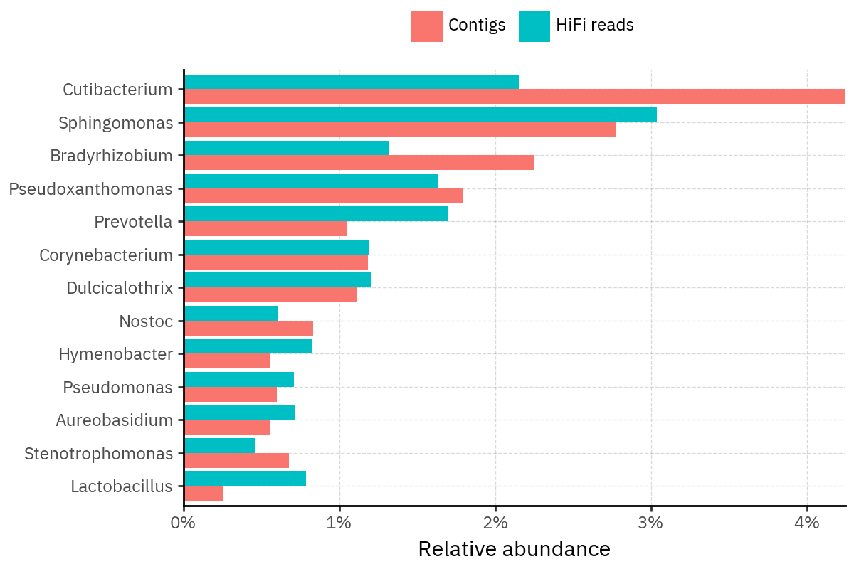
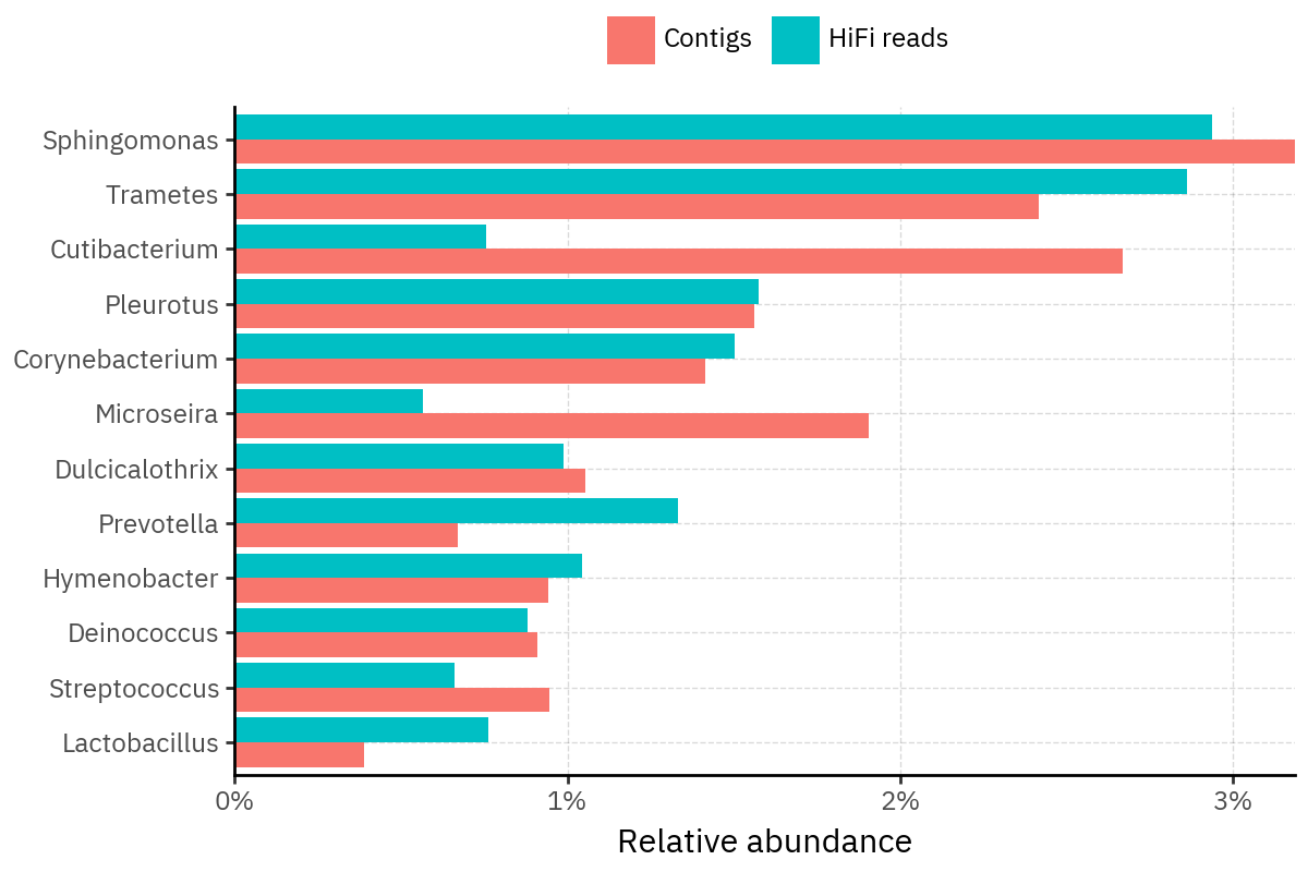
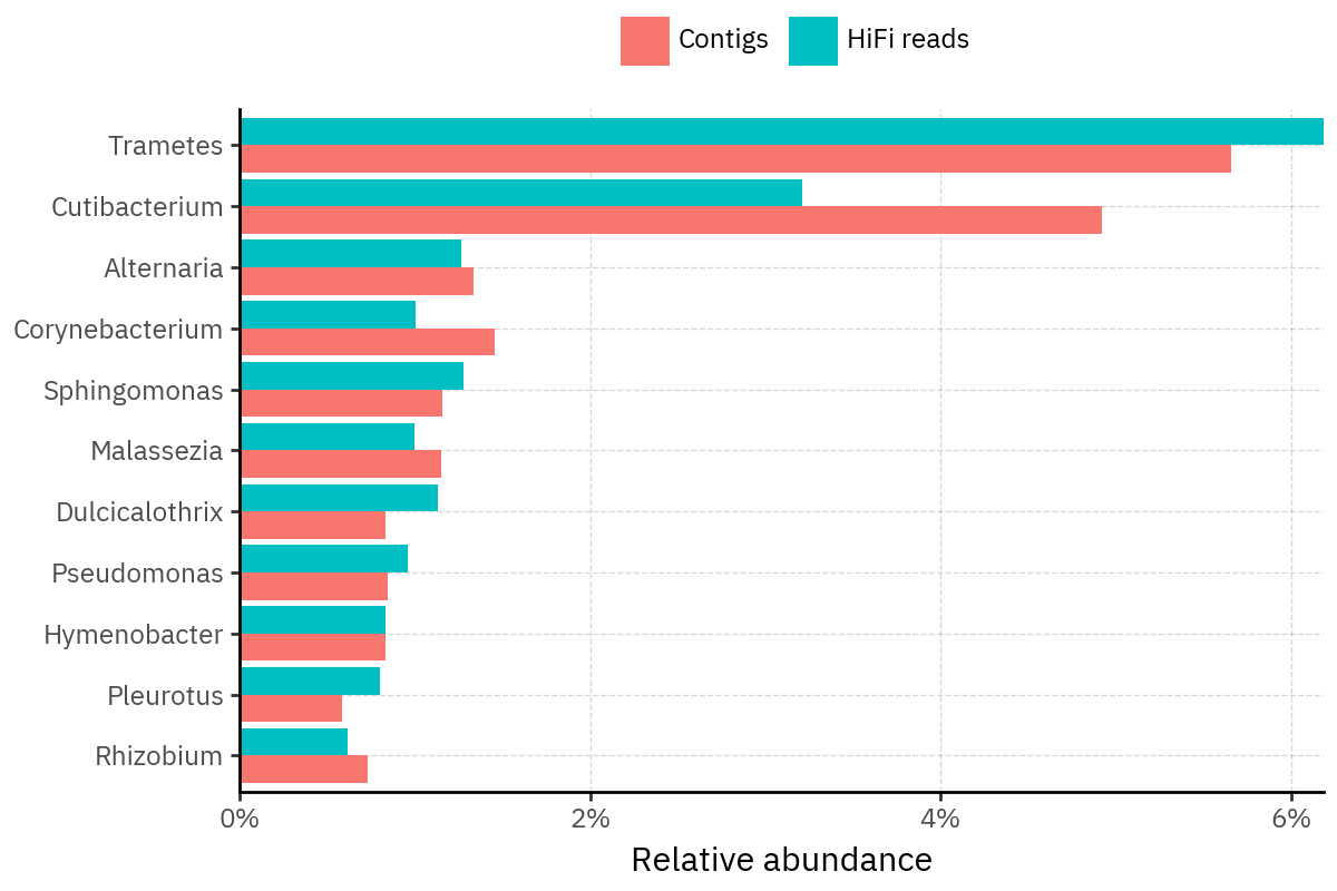
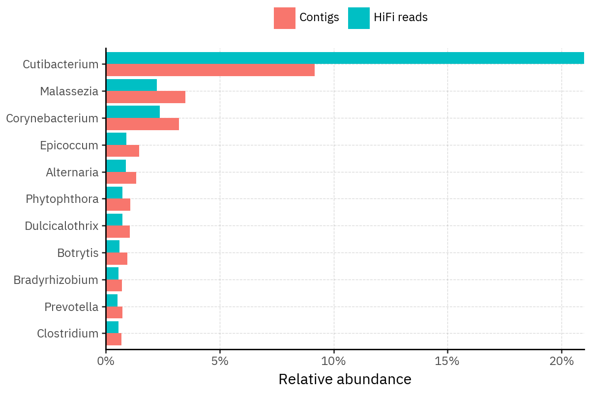
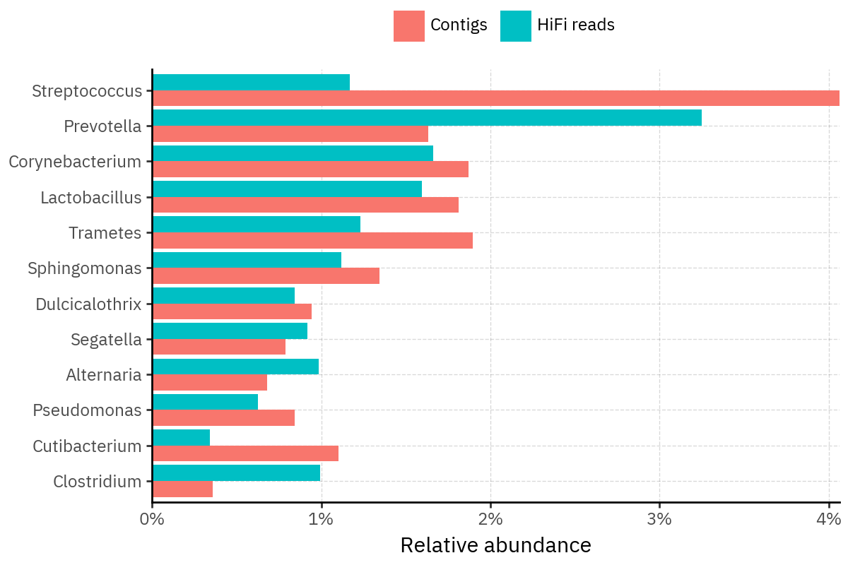
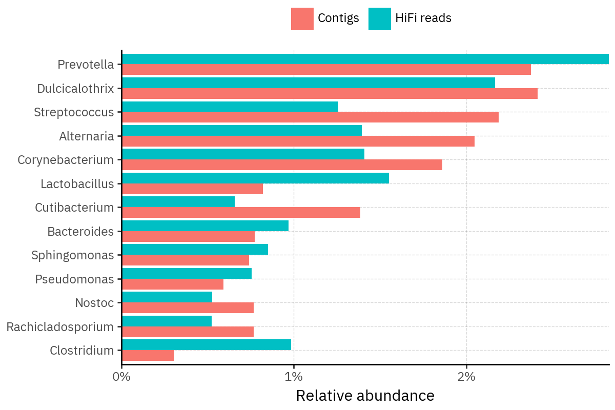
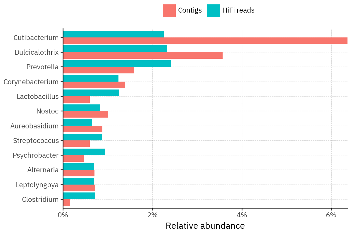
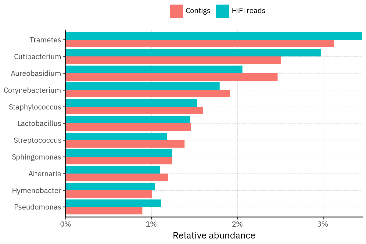
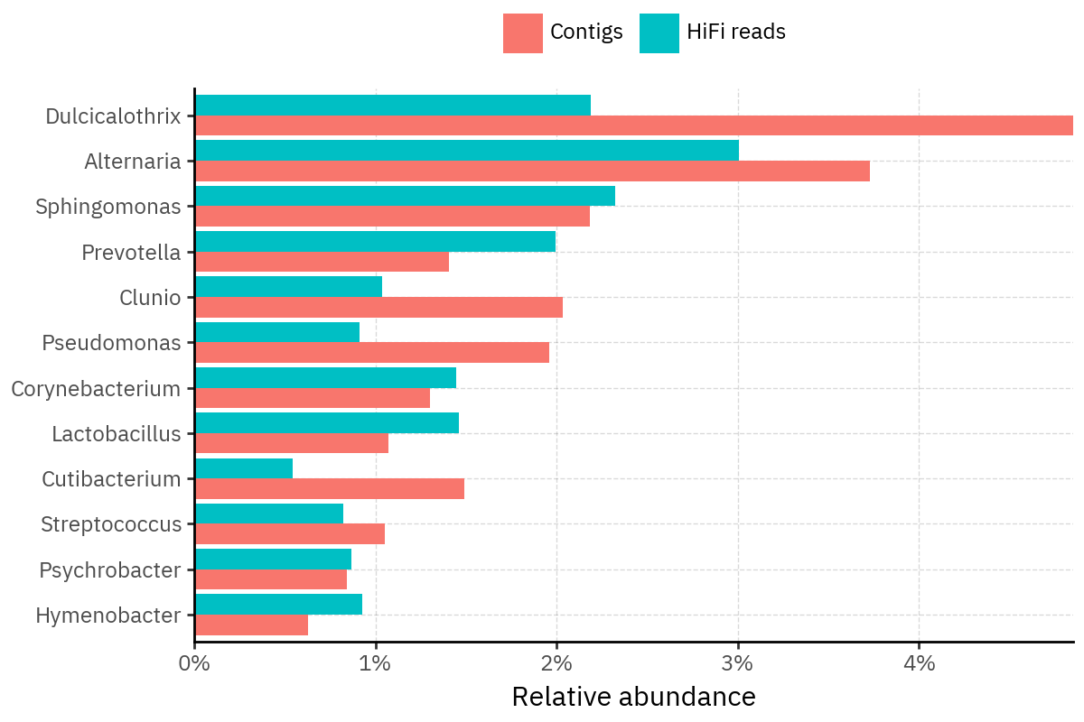
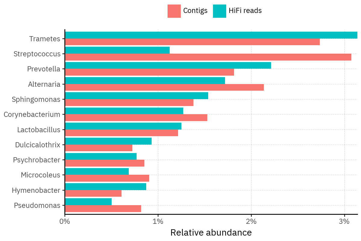
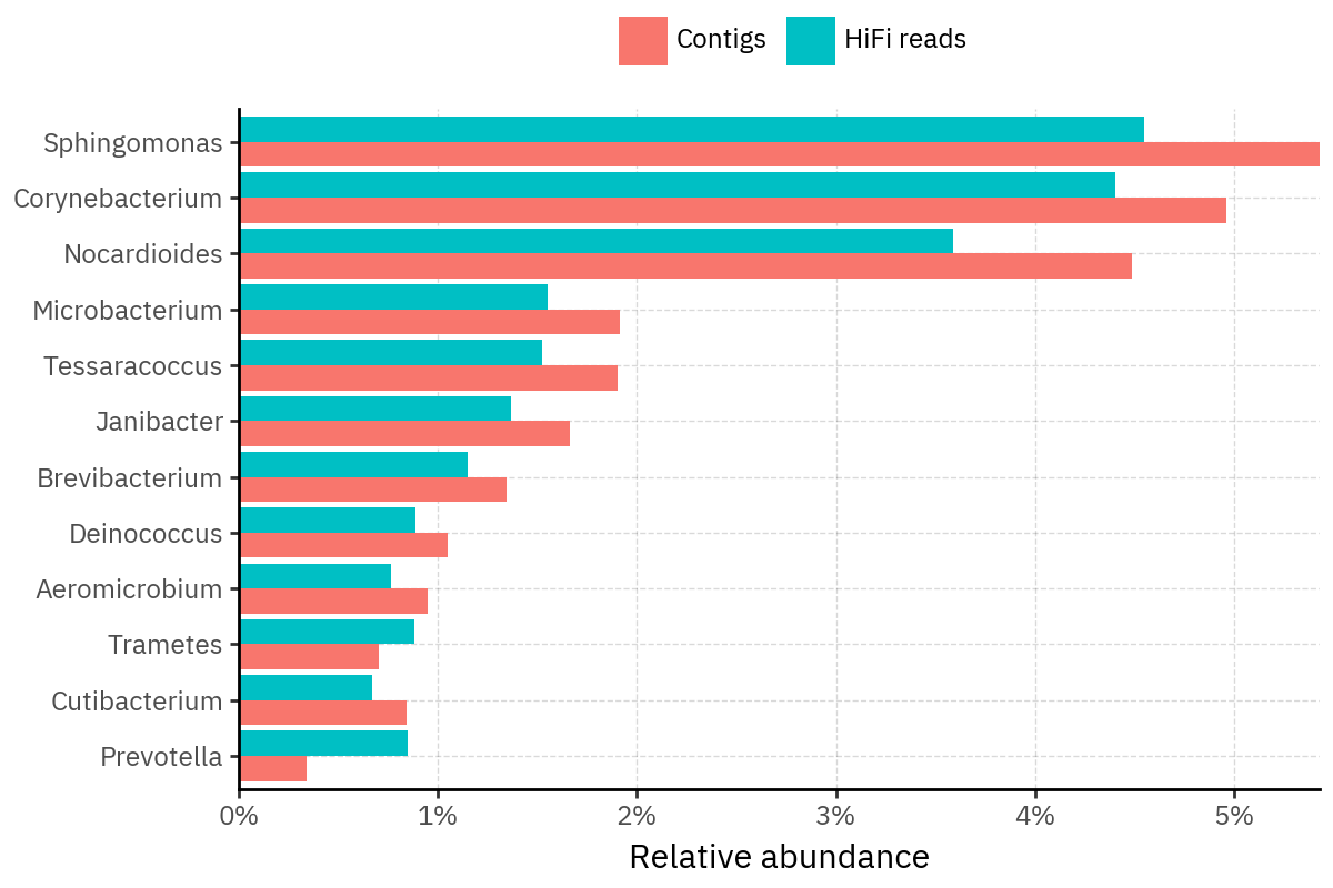
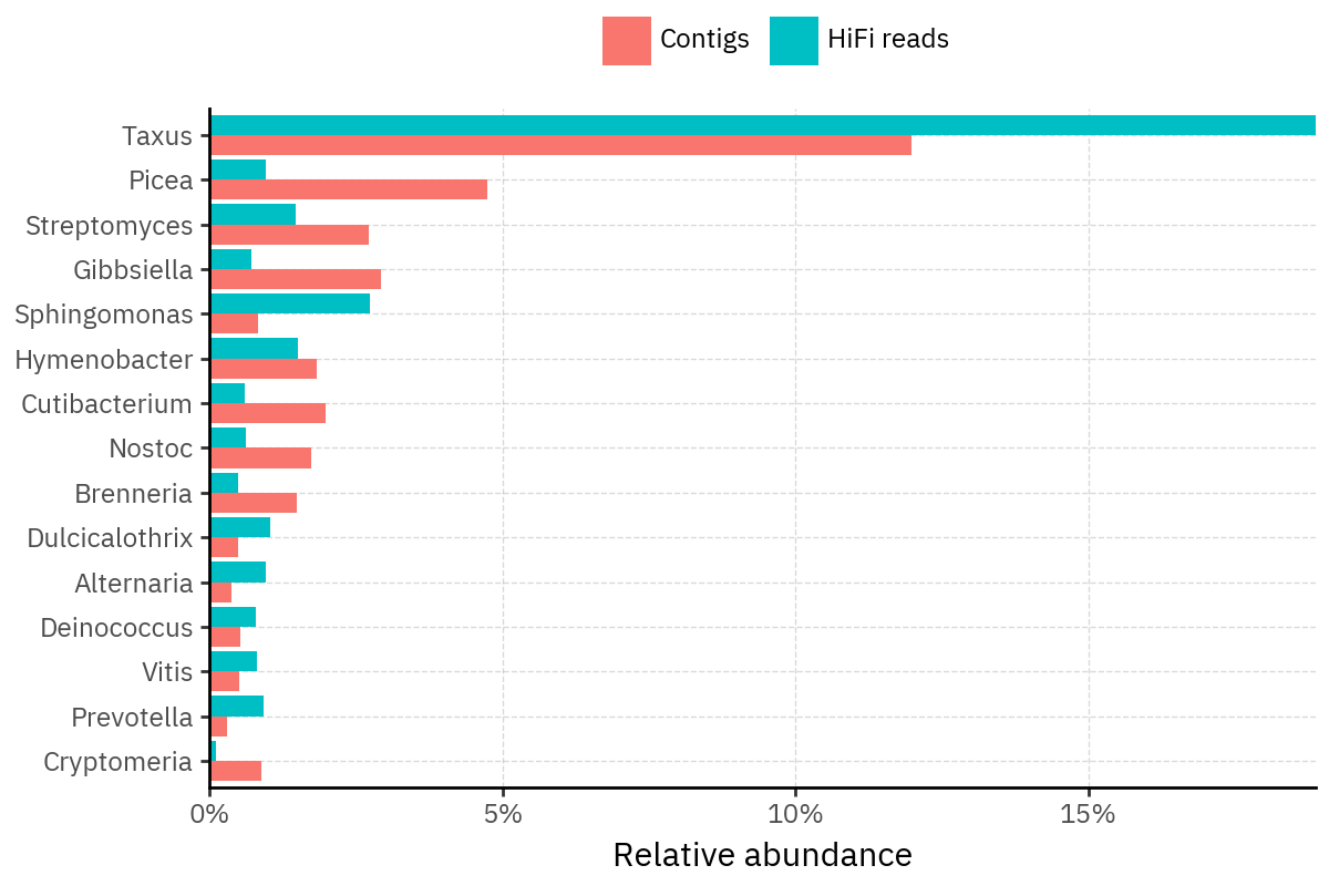
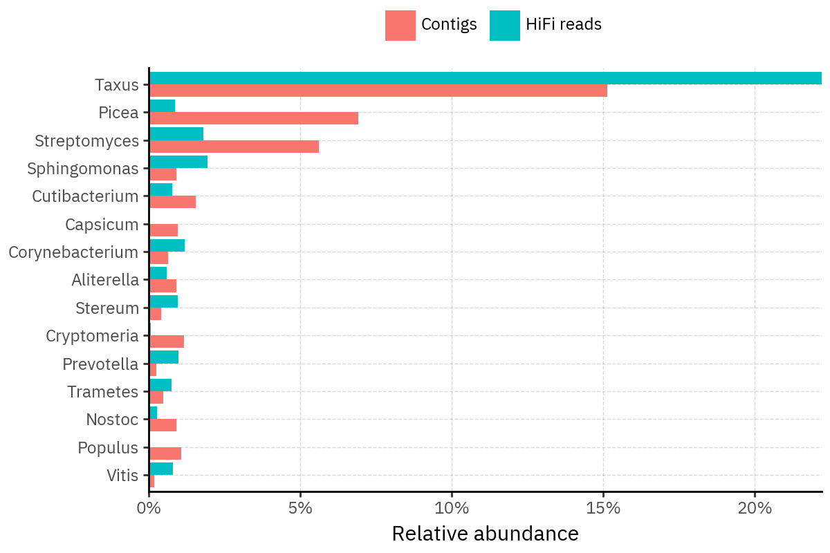
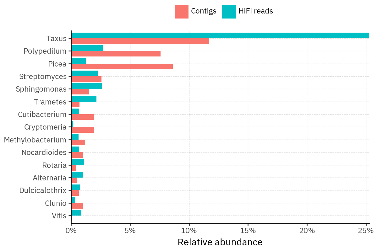
Because species calls can be sensitive to depth of classification, I repeat the same visualization at the genus level. This is the first sanity check for whether apparent disagreements are mostly “species depth” artifacts (as in the Lupinus example) versus true genus-level presence/absence differences.

At genus level, the overlap is generally clearer: samples like KS001 share the same dominant genera (e.g., Bifidobacterium, Alternaria, Cutibacterium), even when individual species proportions differ.

Similarly, KS112 remains strongly dominated by the same genus (Taxus) in both methods, indicating that the main ecological signal is stable and that the species-level differences are mostly about resolution and weighting.

Next step: now that genus-level agreement looks stronger, the most interpretable comparison is to build rank-collapsed abundance tables (Genus and Species), and then quantify method agreement per sample (correlation of abundances, overlap of detected taxa above a small threshold, and stability of the top-k taxa) before moving on to any downstream ecology using the deepest ranks.