This notebook presents a comprehensive analysis of PacBio metagenomic sequencing data from air samples collected in Kumamoto, Japan. The study evaluates the performance of the PacBio META pipeline developed by AIRLAB for environmental DNA (eDNA) analysis in atmospheric samples.
Study Design and Objectives
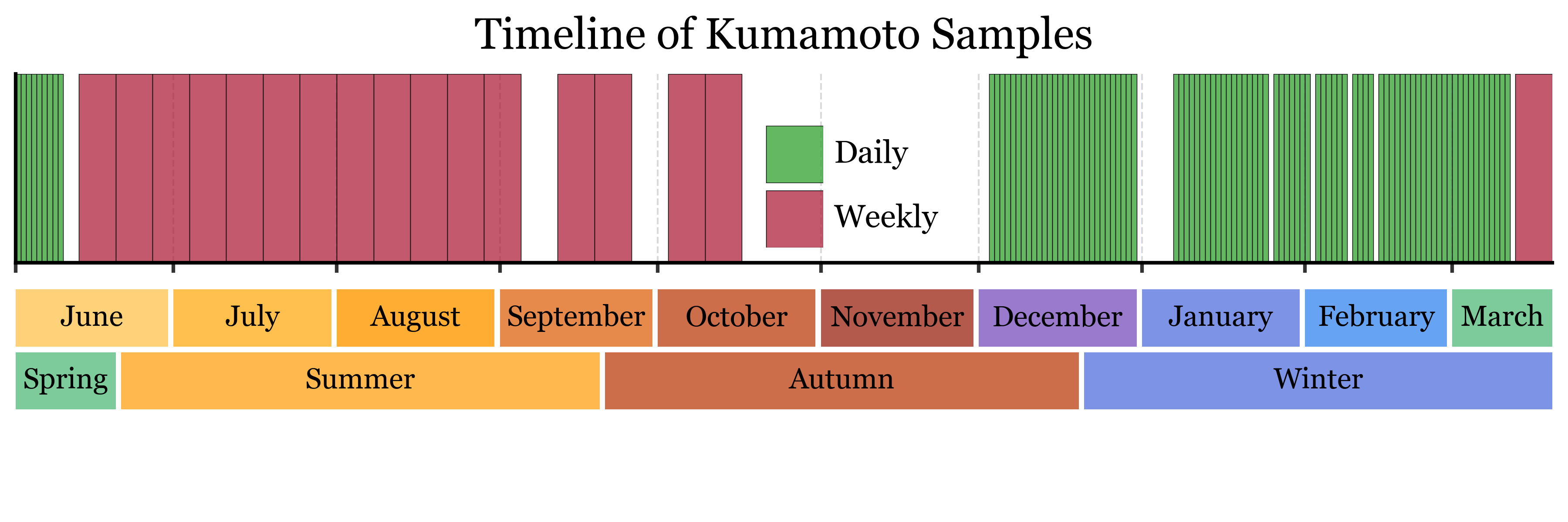
We analyzed air samples collected using different sampling strategies:
Blank samples: Control samples to assess contamination
Daily samples: 24-hour collection periods
Weekly samples: 7-day collection periods
The primary objectives are to:
Evaluate sequencing quality and taxonomic assignment success across sample types
Compare biodiversity patterns between different sampling durations
Assess the pipeline’s ability to capture environmental DNA from major taxonomic groups (Bacteria, Fungi, Metazoa, Viruses)
Investigate temporal patterns in microbial community composition
Table of contents (click to go to each section)
The analysis is structured into several key sections:
Sequencing Statistics: Evaluation of DNA yield, read quality, and sequencing metrics across sample types
Taxonomy Analysis: Comprehensive taxonomic profiling and assignment statistics
The analysis employs both Python and R environments, utilizing established ecological analysis packages (vegan, phyloseq) alongside modern data science tools (pandas, plotnine) to ensure reproducible and statistically robust results.
Key Findings Preview
Initial results suggest significant differences in community composition between sampling strategies, with temporal factors (season, month) showing stronger effects than sampling duration. The pipeline demonstrates high taxonomic assignment success rates, with distinct patterns observed across major taxonomic groups.
Preamble
In this section we load the necessary libraries and set the global parameters for the notebook. It’s irrelevant for the narrative of the analysis but essential for the reproducibility of the results. Since in this case we are using both Python and R, we have a bit of a more complex setup than usual. This includes using the rpy2 package to run R code within the Python environment, as well as ensuring that data is properly passed between the two languages.
Show code imports and presets
Code imports
import osimport warningswarnings.filterwarnings('ignore', category=UserWarning, module='rpy2')# Clean environment variables that cause issues with R# Remove bash functions that R can't parse properlyenv_vars_to_remove = ['BASH_FUNC_ml%%', 'BASH_FUNC_module%%', 'BASH_FUNC_which%%']for var in env_vars_to_remove:if var in os.environ:del os.environ[var]# only if the OS is macOS and R_HOME is not set (otherwise fails...)if os.name =='posix'and os.uname().sysname =='Darwin': os.environ["R_HOME"] ="/Library/Frameworks/R.framework/Resources"%load_ext rpy2.ipython
The rpy2.ipython extension is already loaded. To reload it, use:
  %reload_ext rpy2.ipython
%%R# Load the packageslibrary(dplyr)library(vegan)library(ggplot2)library(phyloseq)library(magrittr)
import reimport numpy as npimport pandas as pdimport plotnine as p9import geopandas as gpdfrom glob import globfrom Bio import Entrezfrom ete3 import NCBITaxafrom collections import defaultdictfrom itables import init_notebook_mode, showfrom plotnine.composition import plot_spacerfrom mizani.labels import label_percent, label_scientific
We have been working on the taxonomic analysis of air samples collected in Kumamoto, Japan, which were subsequently sequenced using PacBio, and which we have processed using the PacBio META pipeline developed in the AIRLAB. The goal of this notebook is to evaluate the results of the pipeline, compare the biodiversity of the samples from the point of view of Bacteria, Fungi, other Metazoa and to assess the ability of the pipeline to properly capture the eDNA present in the environment.
Analysis
Sequencing stats
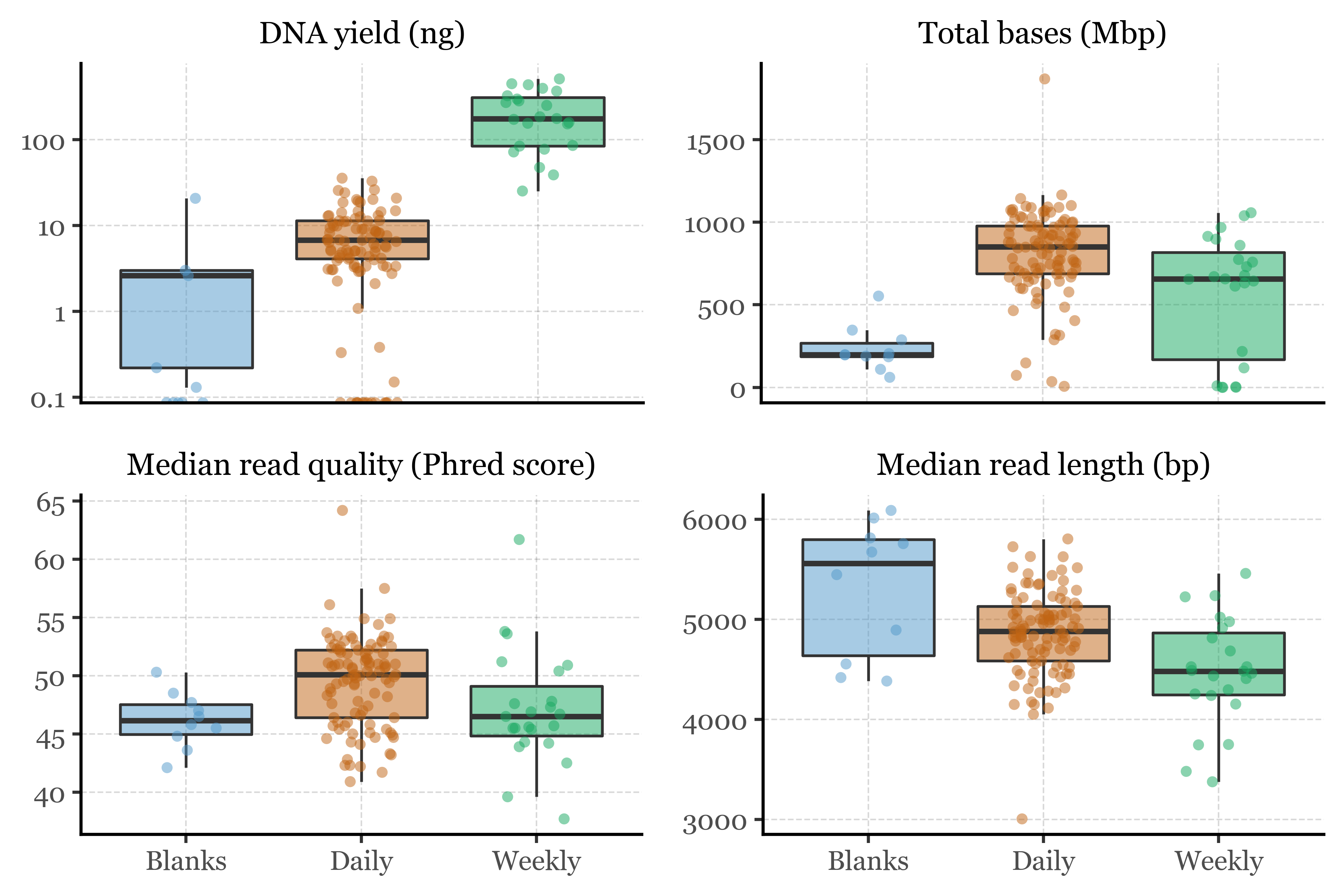
We’ll load the metadata from our filter database and the sequencing metrics from the PacBio pipeline, then merge them to create a single dataframe with all the information needed to examine and compare the results from the blanks, the daily and the weekly samples.
If we compare the results from the blanks, the daily and the weekly samples, we observe the following:
The blanks have lower DNA yield (as expected) which also leads to a lower total bases count. The median read length and quality, however, are similar to the values for the samples, with the highest median read length. This can be explained by the fact that the blanks are not as degraded as the samples, which have been exposed to the environment for longer periods of time.
The daily samples have lower DNA yield than the weekly samples, which is expected since they collected approximately 7 times less air volume. However, this doesn’t appear to affect the total base count, as most likely the sequencing was performed to saturation for all samples.
The observed differences are statistically significant, with a Kruskal-Wallis test showing differences across all four metrics (p-values < 0.001). The post-hoc Dunn’s test shows that the differences are significant between all groups, with the exception of the median read length and quality between the blanks and the daily samples and blanks and weekly samples, respectively:
Statistical Analysis of Sequencing Metrics
%%R -i kumamoto_comps_df -o pairwise_dfkumamoto_comps_df$sample_duration <-as.factor(kumamoto_comps_df$sample_duration)numeric_vars <- c('dna_yield', 'total_bases', 'median_read_length', 'median_read_quality')kruskal_results <- lapply(numeric_vars, function(var) { test <- kruskal.test(kumamoto_comps_df[[var]] ~ kumamoto_comps_df$sample_duration) data.frame( variable = var, statistic = test$statistic, p_value = test$p.value)})significant_vars <- numeric_vars[sapply(kruskal_results, function(x) x$p_value <0.05)]pairwise_df <- lapply(significant_vars, function(var) {# Run Dunn's test dunn_res <- FSA::dunnTest(kumamoto_comps_df[[var]] ~ kumamoto_comps_df$sample_duration, method ="bh")# Extract the "res" table and add the variable name df <- dunn_res$res %>% dplyr::mutate(variable = var)return(df)}) %>% dplyr::bind_rows()
Show Code
(pairwise_df .replace({'variable': {'dna_yield': 'DNA Yield','total_bases': 'Total Bases','median_read_length': 'Median Read Length','median_read_quality': 'Median Read Quality'}}) [['variable', 'Comparison', 'Z', 'P.unadj', 'P.adj']] .style .hide(axis='index') .format(precision=4)# color P.adj < .05 rows in red .apply(lambda x: ['color: red'if v <0.05else''for v in x], subset=['P.adj']))
variable
Comparison
Z
P.unadj
P.adj
DNA Yield
Blanks - Daily
-2.5939
0.0095
0.0095
DNA Yield
Blanks - Weekly
-6.6136
0.0000
0.0000
DNA Yield
Daily - Weekly
-7.1209
0.0000
0.0000
Total Bases
Blanks - Daily
-4.6865
0.0000
0.0000
Total Bases
Blanks - Weekly
-2.2314
0.0257
0.0257
Total Bases
Daily - Weekly
3.0662
0.0022
0.0033
Median Read Length
Blanks - Daily
1.8021
0.0715
0.0715
Median Read Length
Blanks - Weekly
3.4533
0.0006
0.0017
Median Read Length
Daily - Weekly
3.0759
0.0021
0.0031
Median Read Quality
Blanks - Daily
-2.6883
0.0072
0.0215
Median Read Quality
Blanks - Weekly
-0.7613
0.4465
0.4465
Median Read Quality
Daily - Weekly
2.6092
0.0091
0.0136
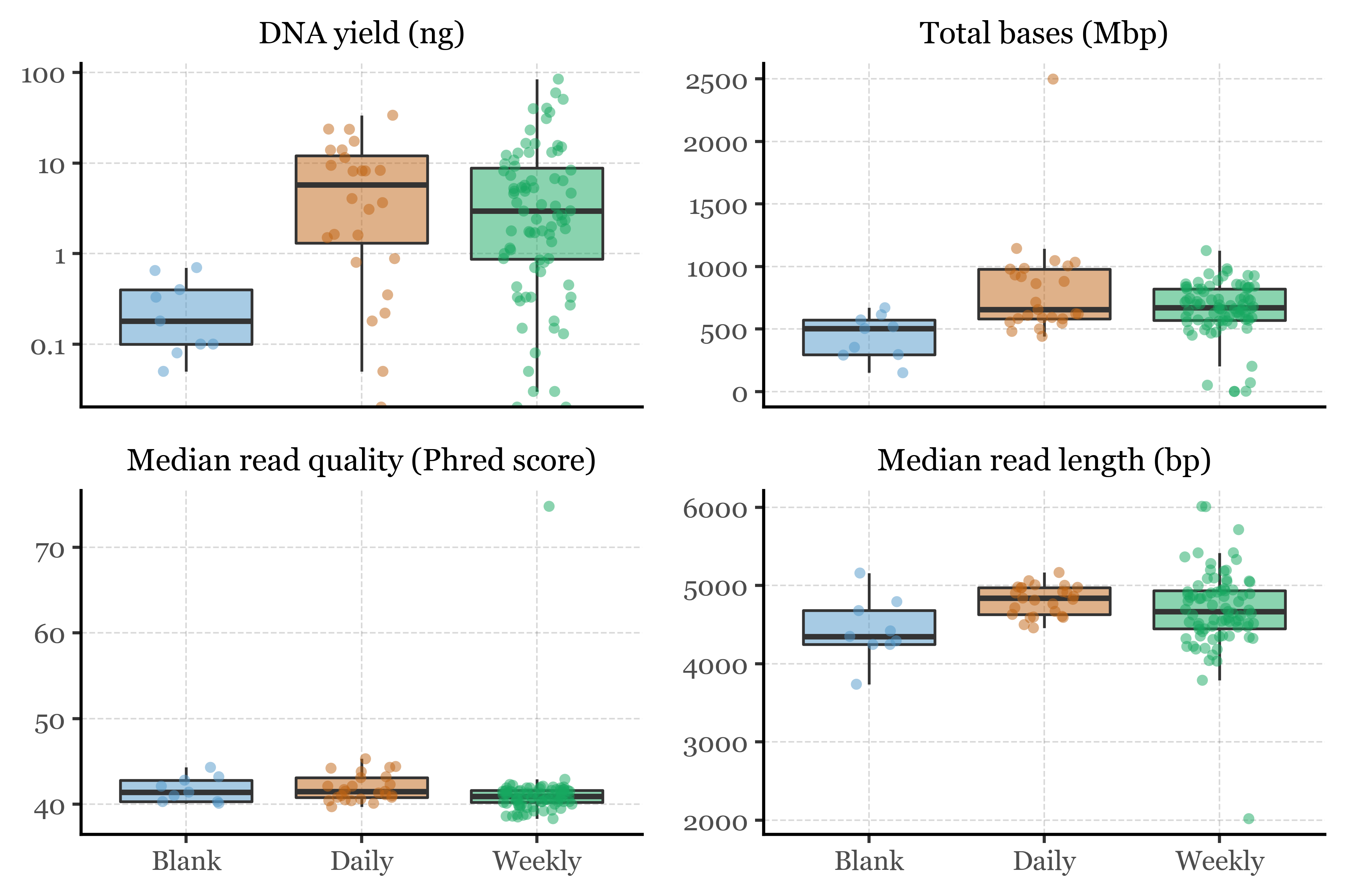
If we run the same comparisons, but now for the Toyama samples, however…
%%R -i toyama_comps_df -o pairwise_toyama_df -o kruskal_results_headertoyama_comps_df$sample_duration <-as.factor(toyama_comps_df$sample_duration)toyama_comps_df$sample_header <-as.factor(toyama_comps_df$sample_header)numeric_vars <- c('dna_yield', 'total_bases', 'median_read_length', 'median_read_quality')kruskal_results <- lapply(numeric_vars, function(var) { test <- kruskal.test(toyama_comps_df[[var]] ~ toyama_comps_df$sample_duration) data.frame( variable = var, statistic = test$statistic, p_value = test$p.value)})significant_vars <- numeric_vars[sapply(kruskal_results, function(x) x$p_value <0.05)]toyama_comps_samples <- toyama_comps_df %>% dplyr::filter(sample_type !='Blank')kruskal_results_header <- lapply(numeric_vars, function(var) { test <- kruskal.test(toyama_comps_samples[[var]] ~ toyama_comps_samples$sample_header) data.frame( variable = var, statistic = test$statistic, p_value = test$p.value)})pairwise_toyama_df <- lapply(significant_vars, function(var) {# Run Dunn's test dunn_res <- FSA::dunnTest(toyama_comps_df[[var]] ~ toyama_comps_df$sample_duration, method ="bh")# Extract the "res" table and add the variable name df <- dunn_res$res %>% dplyr::mutate(variable = var)return(df)}) %>% dplyr::bind_rows()
Show Code
(pairwise_toyama_df .replace({'variable': {'dna_yield': 'DNA Yield','total_bases': 'Total Bases','median_read_length': 'Median Read Length','median_read_quality': 'Median Read Quality'}}) [['variable', 'Comparison', 'Z', 'P.unadj', 'P.adj']] .style .hide(axis='index') .format(precision=4)# color P.adj < .05 rows in red .apply(lambda x: ['color: red'if v <0.05else''for v in x], subset=['P.adj']))
We’ll begin by loading the taxonomic assignments generated by Diamond and the results from the PacBio META pipeline, then merge them into a single dataframe containing all required information. We will then compare the results from the blanks, the daily and the weekly samples to test for differences in biodiversity between the groups.
The analysis output provides a complex .txt file that requires parsing and cleaning to extract the needed information. For now, we will load all the different taxonomic assignments (including Bacteria, Fungi, Metazoa and Viruses) and then merge them into a single dataframe.
blank_files = glob("../data/kumamoto/blanks/*.txt")sample_files = glob("../data/kumamoto/samples/*.txt")all_files = blank_files + sample_filesfeature_tables = []sample_ids = []for file_path in all_files: sample_id = os.path.splitext(os.path.basename(file_path))[0] df_grouped = process_megan_txt(file_path, sample_id=sample_id) feature_tables.append(df_grouped) sample_ids.append(sample_id)# we combine into a single DataFrame (taxa as rows, samples as columns)big_table_KM = pd.concat(feature_tables, axis=1).fillna(0).astype(float)big_table_KM = big_table_KM.T # transposed so samples are rows, taxa are columnsbig_table_KM.index.name ='sample_id'sample_ids = [s.split('_')[0] for s in big_table_KM.index]big_table_KM.index = sample_ids
Since the standard in metagenomics is the usage of the vegan package for ecological data analysis, we will use it to perform some basic analyses on our feature table, including the calculation of alpha and beta diversity metrics.
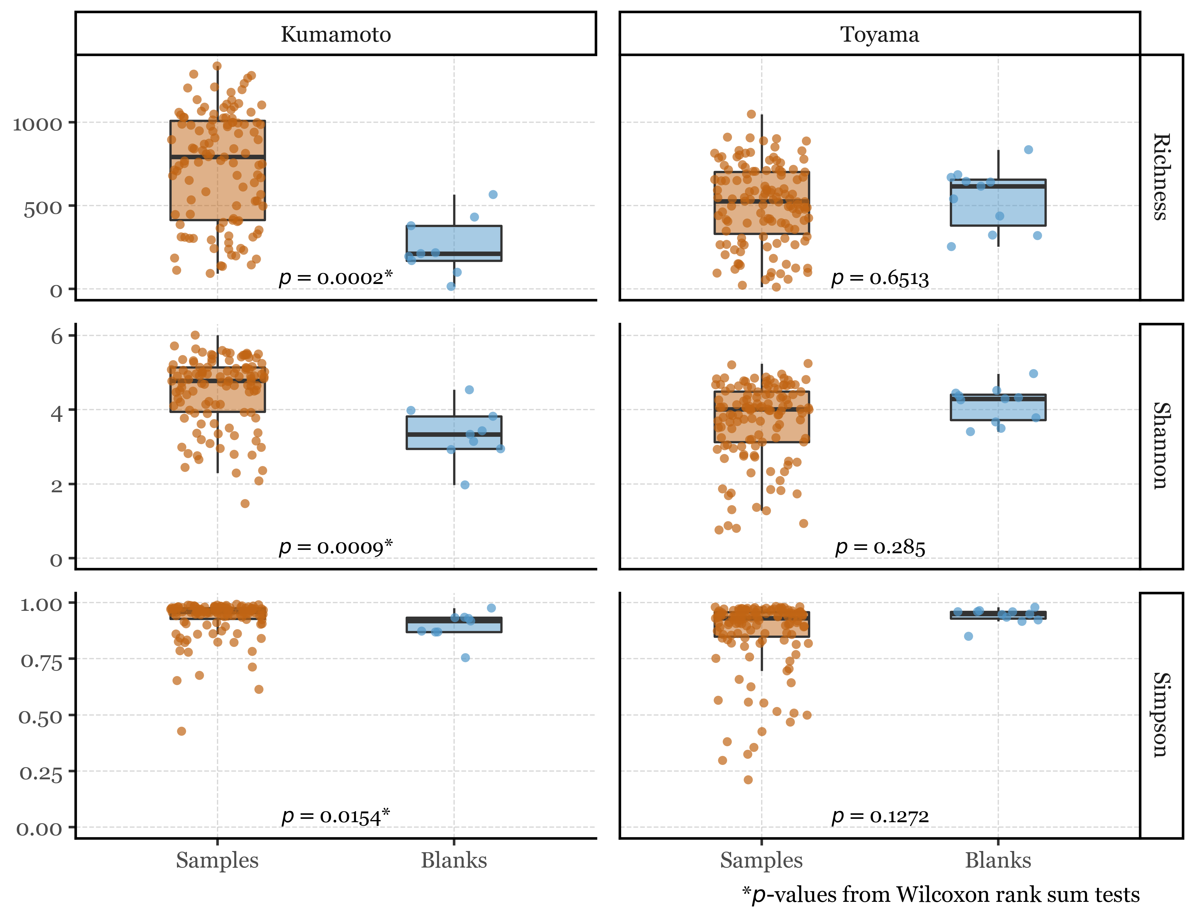
To start, we will compare the alpha diversity metrics between blanks and samples, considering each of the assigned taxa at every taxonomic level as a unique feature. If we do so:
%%R -o diversity_tests_df # We run a wilcoxon test for each metric as read counts are not normally distributedrichness_test_KM <- wilcox.test(richness ~ sample_type, data = diversity_KM)shannon_test_KM <- wilcox.test(shannon ~ sample_type, data = diversity_KM)simpson_test_KM <- wilcox.test(simpson ~ sample_type, data = diversity_KM)richness_test_TY <- wilcox.test(richness ~ sample_type, data = diversity_TY)shannon_test_TY <- wilcox.test(shannon ~ sample_type, data = diversity_TY)simpson_test_TY <- wilcox.test(simpson ~ sample_type, data = diversity_TY)diversity_tests_df <- data.frame( metric = c("Richness", "Shannon", "Simpson", "Richness", "Shannon", "Simpson"), statistic = c(richness_test_KM$statistic, shannon_test_KM$statistic, simpson_test_KM$statistic, richness_test_TY$statistic, shannon_test_TY$statistic, simpson_test_TY$statistic), p_value = c(richness_test_KM$p.value, shannon_test_KM$p.value, simpson_test_KM$p.value, richness_test_TY$p.value, shannon_test_TY$p.value, simpson_test_TY$p.value), location = c(rep("Kumamoto", 3), rep("Toyama", 3)))
The results change by location: In Kumamoto, the samples are, as expected, more diverse than the blanks, with a significant difference in all three metrics (richness, Shannon, and Simpson). However, in Toyama, none of the metrics show significant differences between blanks and samples:
def process_megan_txt(file_path, sample_id=None): df = pd.read_csv( file_path, sep='\t', header=None, names=['taxonomy', 'count'], engine='python' ) df['taxonomy'] = df['taxonomy'].str.strip().str.rstrip(';') df['count'] = df['count'].astype(float)if sample_id isnotNone: df = df.set_index('taxonomy').rename(columns={'count': sample_id})else: df = df.set_index('taxonomy')return df# Gather all sample filesblank_files = glob("../data/kumamoto/blanks/*.txt")sample_files = glob("../data/kumamoto/samples/*.txt")all_files = blank_files + sample_files# Build the abundance tablefeature_tables = []sample_ids = []for file_path in all_files: sample_id = os.path.splitext(os.path.basename(file_path))[0] df_grouped = process_megan_txt(file_path, sample_id=sample_id) feature_tables.append(df_grouped) sample_ids.append(sample_id)# Merge all samples (outer join, fill missing with 0)abundance_table = pd.concat(feature_tables, axis=1).fillna(0).Tabundance_table.index.name ="sample_id"abundance_table.index = [s.split('_')[0] for s in abundance_table.index]tax_split = abundance_table.columns.str.split(';', expand=True)tax_levels = [f'level_{i+1}'for i inrange(tax_split.to_frame().shape[1])]taxonomy_names_df = (tax_split .to_frame() .reset_index(drop=True) .rename(columns=dict((i, f'level_{i+1}') for i inrange(tax_split.to_frame().shape[1]))) .map(lambda x: x.lstrip() ifisinstance(x, str) else x))
def get_complete_taxonomy_lineage(row, ncbi):""" Extract the most specific taxon from a row and get the COMPLETE lineage preserving all NCBI taxonomic ranks, not just the standard 7. """# Get all non-null values from the row (excluding non-taxonomic columns) taxa = [val for val in row if pd.notna(val) and val !=''and val !='NCBI']ifnot taxa:return {}# Start from most specific (rightmost) taxonfor taxon inreversed(taxa):try:# Get taxon ID name_dict = ncbi.get_name_translator([taxon])if taxon in name_dict: taxid = name_dict[taxon][0]# Get COMPLETE lineage (all taxonomic IDs) lineage = ncbi.get_lineage(taxid)# Get ranks and names for all lineage members ranks = ncbi.get_rank(lineage) names = ncbi.get_taxid_translator(lineage)# Create complete taxonomy dictionary with ALL ranks result = {}# Add all ranks found in the lineagefor tid in lineage: rank = ranks[tid] name = names[tid]# Skip 'no rank' entries but keep everything elseif rank !='no rank'and rank !='': result[rank] = name# Also add any intermediate ranks that might be missing# by checking for common NCBI ranks all_possible_ranks = ['superkingdom', 'kingdom', 'subkingdom','superphylum', 'phylum', 'subphylum', 'infraphylum','superclass', 'class', 'subclass', 'infraclass','cohort', 'subcohort', 'superorder', 'order', 'suborder', 'infraorder','parvorder', 'superfamily', 'family', 'subfamily', 'tribe', 'subtribe','genus', 'subgenus', 'species group', 'species subgroup', 'species', 'subspecies', 'strain', 'varietas', 'forma' ]return resultexceptExceptionas e:print(f"Error processing {taxon}: {e}")continuereturn {}def standardize_taxonomy_dataframe(df, ncbi=None):""" Process a taxonomy dataframe and return a standardized version with all available taxonomic ranks preserved. """if ncbi isNone:print("Initializing NCBI taxonomy database...") ncbi = NCBITaxa()# Apply the taxonomy extraction to each row taxonomy_results = []for _, row in df.iterrows(): result = get_complete_taxonomy_lineage(row, ncbi) taxonomy_results.append(result)# Convert to DataFrame df_standardized = pd.DataFrame(taxonomy_results)# Reorder columns by typical taxonomic hierarchy if they exist preferred_order = ['acellular root', 'cellular root', 'domain', 'realm', 'clade','superkingdom', 'kingdom', 'subkingdom','superphylum', 'phylum', 'subphylum', 'infraphylum','superclass', 'class', 'subclass', 'infraclass','cohort', 'subcohort', 'superorder', 'order', 'suborder', 'infraorder','parvorder', 'superfamily', 'family', 'subfamily', 'tribe', 'subtribe','genus', 'subgenus', 'species group', 'species subgroup', 'species', 'subspecies', 'strain', 'varietas', 'forma' ]# Reorder columns based on preferred hierarchy existing_cols = [col for col in preferred_order if col in df_standardized.columns] other_cols = [col for col in df_standardized.columns if col notin preferred_order] new_column_order = existing_cols + other_cols df_standardized = df_standardized[new_column_order]return df_standardizeddef get_taxon_ids_for_best_taxonomy(df_standardized, ncbi=None):""" Get NCBI taxon IDs for the most specific taxonomic rank available in each row. Parameters: df_standardized: DataFrame with standardized taxonomy and 'best_available_taxonomy' column ncbi: NCBITaxa object (optional, will create if not provided) Returns: DataFrame with added taxon ID columns """if ncbi isNone:print("Initializing NCBI taxonomy database...") ncbi = NCBITaxa() df_result = df_standardized.copy()# Add columns for taxon IDs df_result['best_taxonomy_taxid'] = np.nan df_result['best_taxonomy_name'] ='' df_result['best_taxonomy_level'] ='' df_result['taxid_status'] =''# Track success/failureprint("Getting taxon IDs for most specific taxonomic ranks...")# Define hierarchy from most specific to least specific hierarchy = ['subspecies', 'strain', 'varietas', 'forma', # Below species'species', # Species level'species subgroup', 'species group', # Between genus and species'genus', 'subgenus', # Genus level'tribe', 'subtribe', # Above genus'subfamily', 'family', # Family level'order', 'class', 'phylum', # Higher levels'realm', 'clade', 'domain', 'subkingdom', 'superkingdom', 'kingdom','cellular root', 'acellular root'# NCBI ranks ]# Statistics tracking total_rows =len(df_result) success_count =0 failed_names = []for idx, row in df_result.iterrows():# Find the most specific taxonomic level available best_taxon_name =None best_level =Nonefor level in hierarchy:if level in df_result.columns and pd.notna(row[level]) and row[level] !='': best_taxon_name = row[level] best_level = levelbreakif best_taxon_name isNone: df_result.loc[idx, 'taxid_status'] ='no_taxonomy_data'continue# Try to get taxon ID from NCBItry:# Clean the name (remove extra whitespace) clean_name =str(best_taxon_name).strip()# Get taxon ID using ete3 name_dict = ncbi.get_name_translator([clean_name])if clean_name in name_dict andlen(name_dict[clean_name]) >0: taxid = name_dict[clean_name][0] # Take first match# Store results df_result.loc[idx, 'best_taxonomy_taxid'] = taxid df_result.loc[idx, 'best_taxonomy_name'] = clean_name df_result.loc[idx, 'best_taxonomy_level'] = best_level df_result.loc[idx, 'taxid_status'] ='success' success_count +=1else: df_result.loc[idx, 'taxid_status'] ='name_not_found' failed_names.append(clean_name)exceptExceptionas e: df_result.loc[idx, 'taxid_status'] =f'error: {str(e)}' failed_names.append(best_taxon_name)# Print summary statisticsprint(f"\n=== TAXON ID RETRIEVAL SUMMARY ===")print(f"Total entries processed: {total_rows}")print(f"Successfully retrieved taxon IDs: {success_count}")print(f"Success rate: {(success_count/total_rows)*100:.1f}%")# Show status breakdown status_counts = df_result['taxid_status'].value_counts()print(f"\nStatus breakdown:")for status, count in status_counts.items():print(f" {status}: {count}")# Show most common failed namesif failed_names:print(f"\nTop 10 most common failed lookups:") failed_series = pd.Series(failed_names)for name, count in failed_series.value_counts().head(10).items():print(f" {name}: {count}")return df_result
Getting taxon IDs for most specific taxonomic ranks...

=== TAXON ID RETRIEVAL SUMMARY ===
Total entries processed: 14391
Successfully retrieved taxon IDs: 14388
Success rate: 100.0%

Status breakdown:
  success: 14388
  no_taxonomy_data: 3
Define and validate species name standardization functions
def standardize_species_names(df):""" Standardize species names across the entire taxonomy dataframe """import redef fix_species(row):# If species already exists and looks good, keep itif pd.notna(row['species']) and row['species'] !=''andnot'unclassified'instr(row['species']).lower():return row['species']# Only try to fix if best_taxonomy_level is at genus level or below genus_and_below_levels = ['genus', 'subgenus', 'species group', 'species subgroup', 'species', 'subspecies', 'strain', 'varietas', 'forma']if row['best_taxonomy_level'] notin genus_and_below_levels:return"Unclassified"# Try to extract from best_taxonomy_nameif pd.notna(row['best_taxonomy_name']): name =str(row['best_taxonomy_name']).strip()# Pattern for proper binomial nomenclature binomial_patterns = [r'^([A-Z][a-z]+)\s+([a-z]+)$', # Simple binomialr'^([A-Z][a-z]+)\s+([a-z]+)\s+([a-z]+)$', # Trinomial (subspecies)r'^([A-Z][a-z]+)\s+(sp\.)\s+([A-Za-z0-9_-]+)$', # Genus sp. strain ]for pattern in binomial_patterns: match = re.match(pattern, name)if match: genus_from_name = match.group(1) species_epithet = match.group(2)# Skip non-specific epithets that aren't real species names non_specific_epithets = ['group', 'clade', 'complex', 'cluster', 'assemblage', 'section', 'series']if species_epithet.lower() in non_specific_epithets:return"Unclassified"# Verify genus consistencyif pd.notna(row['genus']) and row['genus'] !='':if genus_from_name == row['genus']:if species_epithet =='sp.':returnf"{genus_from_name}{species_epithet}{match.group(3)}"else:returnf"{genus_from_name}{species_epithet}"else:# Use what we foundif species_epithet =='sp.':returnf"{genus_from_name}{species_epithet}{match.group(3)}"else:returnf"{genus_from_name}{species_epithet}"return"Unclassified"return df.assign(species=df.apply(fix_species, axis=1))def validate_species_extraction(df):""" Check how many species were recovered vs missing """ before_fix = df['species'].notna().sum() df_fixed = standardize_species_names(df) after_fix = (df_fixed['species'] !='Unclassified').sum()print(f"Species names before fix: {before_fix}")print(f"Species names after fix: {after_fix}")print(f"Improvement: {after_fix - before_fix} additional species recovered")# Show examples of what was fixed fixed_examples = (df_fixed[(df['species'].isna() | (df['species'] =='')) & (df_fixed['species'] !='Unclassified')])for _, row in fixed_examples.iterrows():print(f"{row['best_taxonomy_level']}: {row['best_taxonomy_name']} -> Fixed Species: {row['species']}")validate_species_extraction(taxonomy_with_ids)
Species names before fix: 10840
Species names after fix: 10868
Improvement: 28 additional species recovered
species subgroup: Stutzerimonas stutzeri subgroup -> Fixed Species: Stutzerimonas stutzeri
species group: Burkholderia cepacia complex -> Fixed Species: Burkholderia cepacia
species group: Alternaria alternata complex -> Fixed Species: Alternaria alternata
species group: Pseudomonas aeruginosa group -> Fixed Species: Pseudomonas aeruginosa
species group: Pseudomonas fluorescens group -> Fixed Species: Pseudomonas fluorescens
species group: Pseudomonas syringae group -> Fixed Species: Pseudomonas syringae
species subgroup: Stutzerimonas stutzeri subgroup -> Fixed Species: Stutzerimonas stutzeri
species group: Agrobacterium tumefaciens complex -> Fixed Species: Agrobacterium tumefaciens
species group: Stutzerimonas stutzeri group -> Fixed Species: Stutzerimonas stutzeri
species group: Enterobacter cloacae complex -> Fixed Species: Enterobacter cloacae
species group: Streptococcus anginosus group -> Fixed Species: Streptococcus anginosus
species group: Citrobacter freundii complex -> Fixed Species: Citrobacter freundii
species group: Pseudomonas putida group -> Fixed Species: Pseudomonas putida
species group: Bacillus subtilis group -> Fixed Species: Bacillus subtilis
species subgroup: Bacillus amyloliquefaciens group -> Fixed Species: Bacillus amyloliquefaciens
species group: Bacillus cereus group -> Fixed Species: Bacillus cereus
species group: Rhodococcus erythropolis group -> Fixed Species: Rhodococcus erythropolis
species group: Enterobacter cloacae complex -> Fixed Species: Enterobacter cloacae
species group: Mycobacterium simiae complex -> Fixed Species: Mycobacterium simiae
species group: Amycolatopsis methanolica group -> Fixed Species: Amycolatopsis methanolica
species group: Pseudomonas aeruginosa group -> Fixed Species: Pseudomonas aeruginosa
species group: Vibrio harveyi group -> Fixed Species: Vibrio harveyi
species group: Mycobacterium tuberculosis complex -> Fixed Species: Mycobacterium tuberculosis
species group: Pseudomonas chlororaphis group -> Fixed Species: Pseudomonas chlororaphis
species group: Prauserella coralliicola group -> Fixed Species: Prauserella coralliicola
species group: Stenotrophomonas maltophilia group -> Fixed Species: Stenotrophomonas maltophilia
species group: Streptomyces violaceusniger group -> Fixed Species: Streptomyces violaceusniger
species group: Streptococcus dysgalactiae group -> Fixed Species: Streptococcus dysgalactiae
Second entry belongs to unclassified_entries -> unclassified_sequences -> environmental_samples so with a search in NCBI’s taxonomy browser we can find that its taxid is 151659:
This taxonomy ID mapping will allow us to keep a single column with the taxonomic IDs, which we will be able to later on use for further analyses without carrying the full taxonomy lineage around.
cellular root     cellular organisms
domain                      Bacteria
kingdom               Pseudomonadati
phylum                Pseudomonadota
class            Alphaproteobacteria
order               Sphingomonadales
family             Sphingomonadaceae
genus                   Sphingomonas
Name: 2329, dtype: object
taxonomy_names_df.iloc[1886]
level_1                          NCBI
level_2            cellular organisms
level_3                      Bacteria
level_4                Proteobacteria
level_5           Alphaproteobacteria
level_6              Sphingomonadales
level_7             Sphingomonadaceae
level_8                  Sphingomonas
level_9     unclassified Sphingomonas
level_10        Sphingomonas sp. YJ09
level_11                          NaN
level_12                          NaN
level_13                          NaN
level_14                          NaN
level_15                          NaN
level_16                          NaN
level_17                          NaN
level_18                          NaN
level_19                          NaN
level_20                          NaN
level_21                          NaN
level_22                          NaN
level_23                          NaN
level_24                          NaN
level_25                          NaN
level_26                          NaN
level_27                          NaN
level_28                          NaN
level_29                          NaN
level_30                          NaN
level_31                          NaN
level_32                          NaN
level_33                          NaN
level_34                          NaN
level_35                          NaN
level_36                          NaN
level_37                          NaN
Name: 1886, dtype: object
Run 0 stress 0.1735855
Run 1 stress 0.1820435
Run 2 stress 0.1839393
Run 3 stress 0.1769141
Run 4 stress 0.1763525
Run 5 stress 0.1865404
Run 6 stress 0.2112716
Run 7 stress 0.1885427
Run 8 stress 0.1888116
Run 9 stress 0.1930841
Run 10 stress 0.1981002
Run 11 stress 0.1703204
... New best solution
... Procrustes: rmse 0.05147571  max resid 0.2497888
Run 12 stress 0.1750515
Run 13 stress 0.1950641
Run 14 stress 0.181364
Run 15 stress 0.188554
Run 16 stress 0.1781962
Run 17 stress 0.1788396
Run 18 stress 0.1866084
Run 19 stress 0.1831665
Run 20 stress 0.1757994
Run 21 stress 0.1773205
Run 22 stress 0.1755386
Run 23 stress 0.1822862
Run 24 stress 0.185336
Run 25 stress 0.1772682
Run 26 stress 0.1836586
Run 27 stress 0.198846
Run 28 stress 0.2094546
Run 29 stress 0.1739281
Run 30 stress 0.1742009
Run 31 stress 0.1820799
Run 32 stress 0.1784877
Run 33 stress 0.1684748
... New best solution
... Procrustes: rmse 0.01739192  max resid 0.1466545
Run 34 stress 0.1838412
Run 35 stress 0.1764085
Run 36 stress 0.1713718
Run 37 stress 0.1822316
Run 38 stress 0.1756282
Run 39 stress 0.1726824
Run 40 stress 0.1847255
Run 41 stress 0.1734816
Run 42 stress 0.1902603
Run 43 stress 0.1752344
Run 44 stress 0.1773065
Run 45 stress 0.2095513
Run 46 stress 0.167005
... New best solution
... Procrustes: rmse 0.01698972  max resid 0.1219746
Run 47 stress 0.191925
Run 48 stress 0.1710904
Run 49 stress 0.1897483
Run 50 stress 0.1793241
Run 51 stress 0.1789115
Run 52 stress 0.1704334
Run 53 stress 0.1745534
Run 54 stress 0.1842467
Run 55 stress 0.1958116
Run 56 stress 0.1789141
Run 57 stress 0.1745232
Run 58 stress 0.176365
Run 59 stress 0.1677557
Run 60 stress 0.1875669
Run 61 stress 0.1739599
Run 62 stress 0.1811732
Run 63 stress 0.1791551
Run 64 stress 0.2114635
Run 65 stress 0.1949473
Run 66 stress 0.1712527
Run 67 stress 0.1954034
Run 68 stress 0.1785225
Run 69 stress 0.1762311
Run 70 stress 0.1803207
Run 71 stress 0.1699237
Run 72 stress 0.1977597
Run 73 stress 0.1774345
Run 74 stress 0.1808974
Run 75 stress 0.1788601
Run 76 stress 0.1844365
Run 77 stress 0.2011627
Run 78 stress 0.1761189
Run 79 stress 0.179456
Run 80 stress 0.1814798
Run 81 stress 0.2100013
Run 82 stress 0.1853572
Run 83 stress 0.1677553
Run 84 stress 0.18513
Run 85 stress 0.1713016
Run 86 stress 0.1660708
... New best solution
... Procrustes: rmse 0.01345051  max resid 0.12158
Run 87 stress 0.1829012
Run 88 stress 0.165895
... New best solution
... Procrustes: rmse 0.007187102  max resid 0.07689487
Run 89 stress 0.2106426
Run 90 stress 0.1854206
Run 91 stress 0.1818669
Run 92 stress 0.190312
Run 93 stress 0.1728266
Run 94 stress 0.1658331
... New best solution
... Procrustes: rmse 0.008056262  max resid 0.07751266
Run 95 stress 0.1765695
Run 96 stress 0.1811998
Run 97 stress 0.1752568
Run 98 stress 0.1746976
Run 99 stress 0.1830565
Run 100 stress 0.1797655
*** Best solution was not repeated -- monoMDS stopping criteria:
     1: no. of iterations >= maxit
    99: stress ratio > sratmax
Run 0 stress 0.1440462
Run 1 stress 0.163319
Run 2 stress 0.1766129
Run 3 stress 0.1449615
Run 4 stress 0.1594438
Run 5 stress 0.1440455
... New best solution
... Procrustes: rmse 0.0001728937  max resid 0.001364318
... Similar to previous best
Run 6 stress 0.1449019
Run 7 stress 0.1440189
... New best solution
... Procrustes: rmse 0.001621551  max resid 0.01392724
Run 8 stress 0.1440189
... New best solution
... Procrustes: rmse 5.081942e-06  max resid 2.545541e-05
... Similar to previous best
Run 9 stress 0.144902
Run 10 stress 0.1440189
... Procrustes: rmse 3.392733e-06  max resid 2.902543e-05
... Similar to previous best
Run 11 stress 0.1440455
... Procrustes: rmse 0.001630253  max resid 0.01394254
Run 12 stress 0.1547519
Run 13 stress 0.1694775
Run 14 stress 0.1440455
... Procrustes: rmse 0.001630834  max resid 0.0139466
Run 15 stress 0.1617539
Run 16 stress 0.1449609
Run 17 stress 0.1800464
Run 18 stress 0.1440462
... Procrustes: rmse 0.001630917  max resid 0.01393746
Run 19 stress 0.1449015
Run 20 stress 0.1449015
*** Best solution repeated 2 times
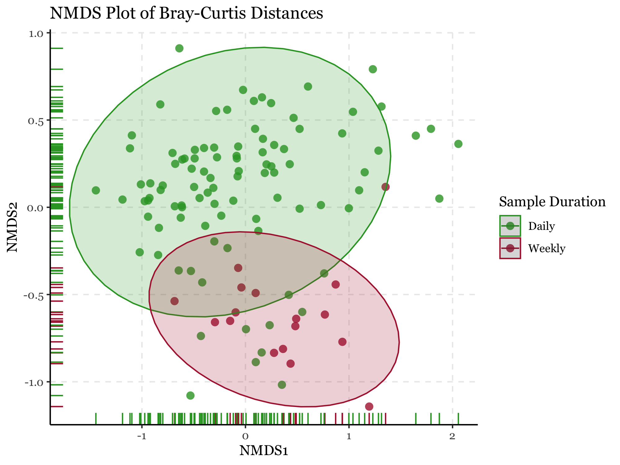
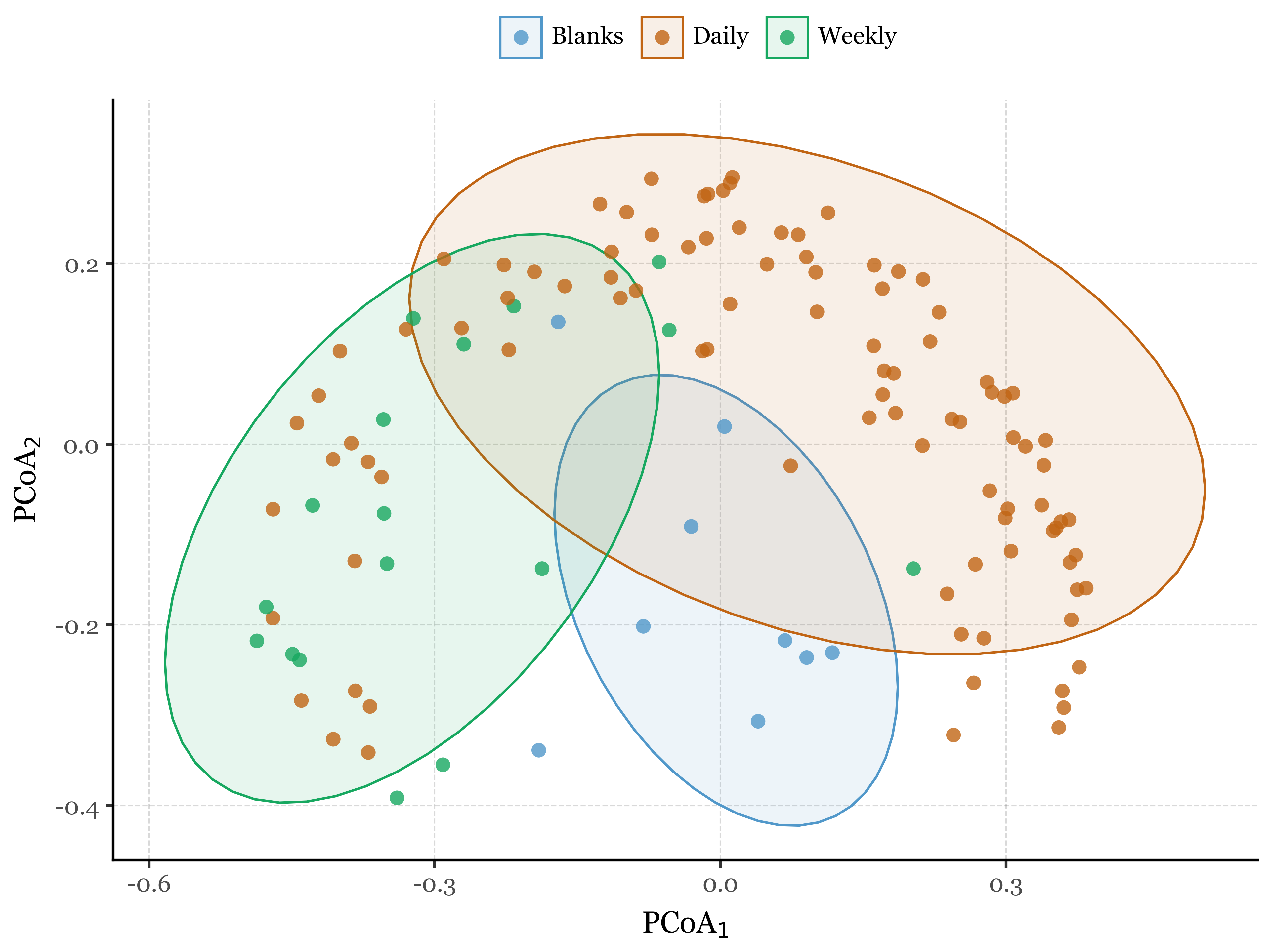
Example of working ggplot2 plot with rpy2 and R magic
I am just leaving this as an example of how to generate plots in R directly while controlling the resolution and size of the output image. I can’t seem to be able to do it directly with the %%R cell magic but using the png() function works fine.
%%R -i nmds_no_blanks_df -i kumamoto_metadata_no_blanks# Plot NMDSpng("nmds_plot.png", res =300, width=2000, height=1500)ggplot(nmds_no_blanks_df, aes(x = NMDS1, y = NMDS2, color = duration)) + geom_point(size =3, alpha =0.8, stroke=0) + scale_color_manual(values=c("#30a12e", "#ae213b")) + scale_fill_manual(values=c("#30a12e", "#ae213b")) + geom_rug() + stat_ellipse(aes(fill = sample_duration), alpha =0.2, level =0.95, geom='polygon') + guides(fill=FALSE) + labs( title ="NMDS Plot of Bray-Curtis Distances", x ="NMDS1", y ="NMDS2", color ="Sample Duration") + theme_classic() + theme( text = element_text(family ="Georgia"), panel.grid.major = element_line(linetype=2) )ggsave("nmds_plot.png")dev.off()
Saving 6.67 x 5 in image
quartz_off_screen
                2
from IPython.display import ImageImage('nmds_plot.png')
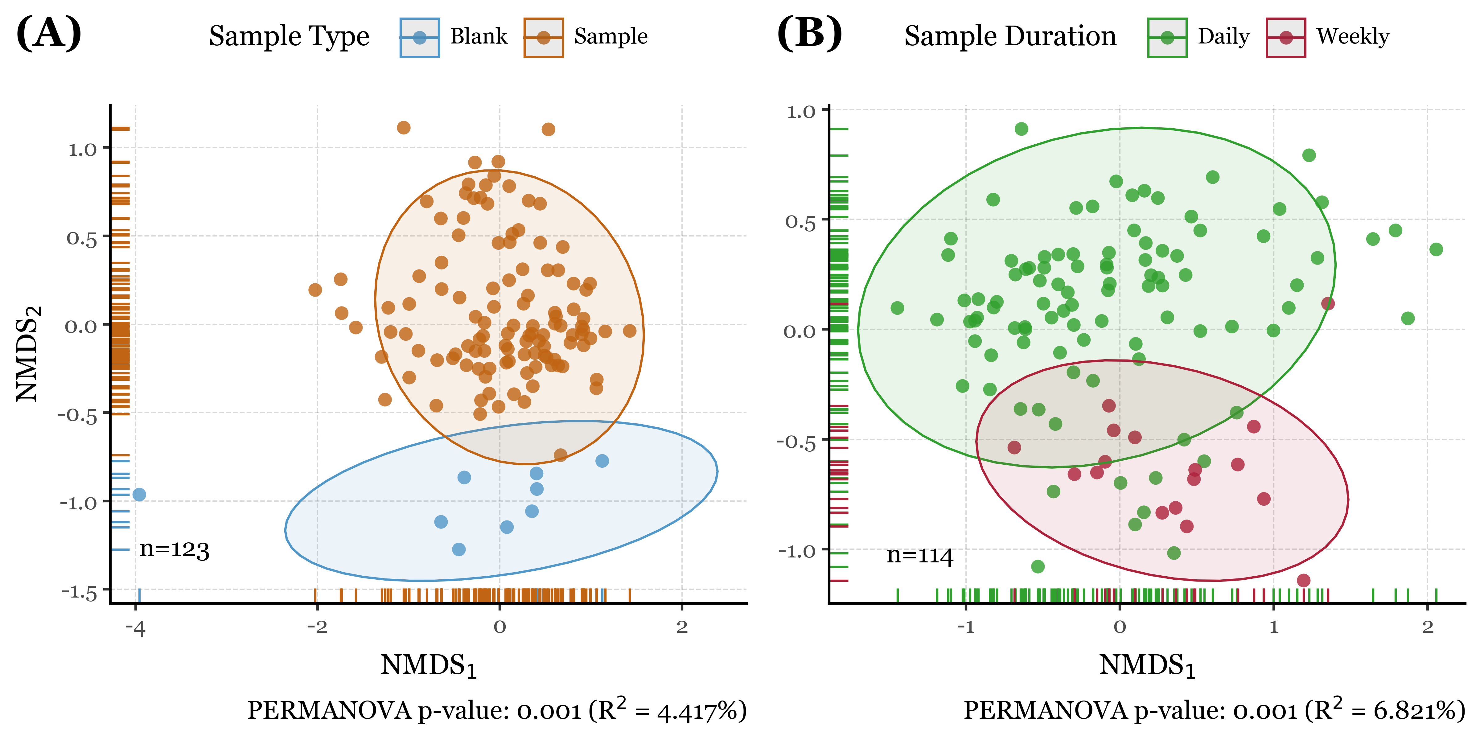
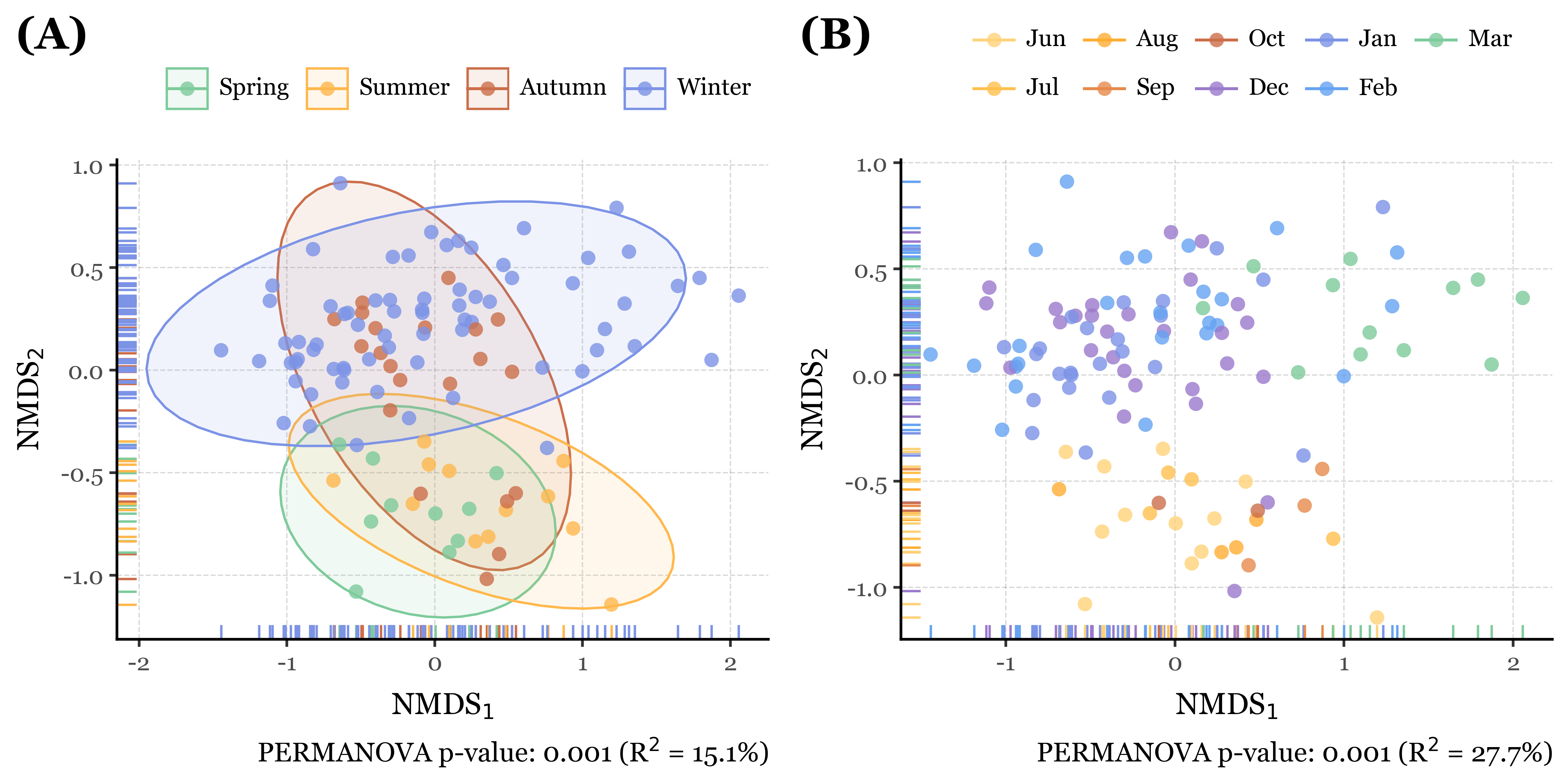
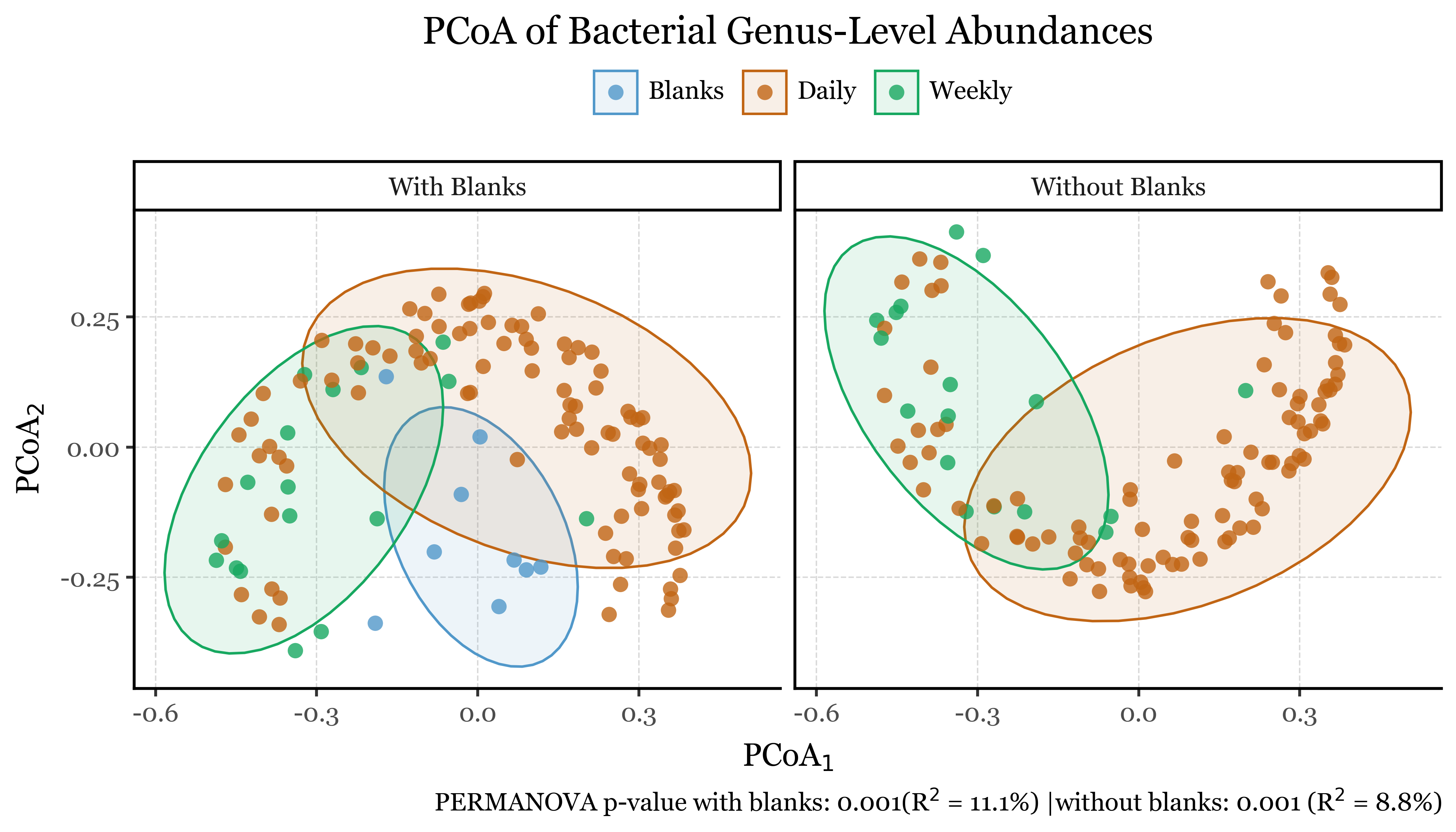
As shown in the results (aside from the satisfaction of finally being able to programmatically generate labeled compositions with plotnine v.0.15.0), the NMDS plots reveal interesting patterns in the data which are confirmed by the PERMANOVA results.
The blanks and actual samples are clearly separated in NMDS space, and significantly different from each other according to the PERMANOVA results (p = 0.001).
As for the sample duration, it also seems have an effect on the composition of the samples, with week-long samples being more similar to each other than to the 24h samples, which are more dispersed in NMDS space. The PERMANOVA results confirm this as well (p = 0.001).
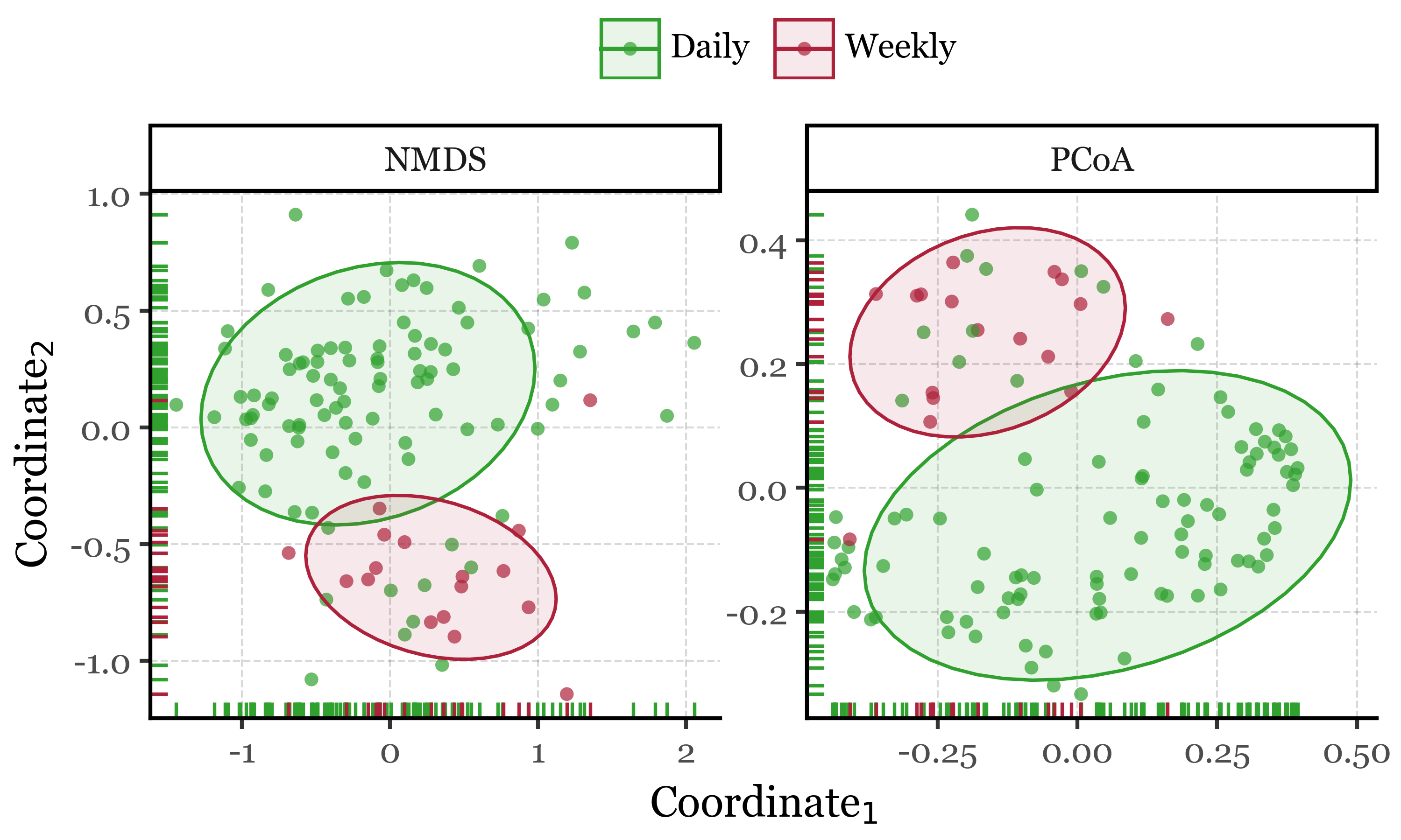
If we now go ahead and color the NMDS plots by season and month, and run the PERMANOVA tests on the same variables, we can see how actually the season and month of the year have a much stronger effect on the composition of the samples than the sample duration, with p = 0.001 for both cases but explaining roughly a 15% and 27% of the variance in community composition, respectively, compared to a mere 7% for the sample duration.
The results are quite clear and consistent, with time being as far as we can tell the main driver of community composition changes in the samples. However, until now we have included every taxonomic level, mixing Bacteria, Fungi, Metazoa and Viruses in the same analysis, which is not ideal since we know that these groups have very different ecological and evolutionary dynamics, and thus an individual analysis of each group might be more informative and reveal different patterns in the data we might not see otherwise.
Big clades
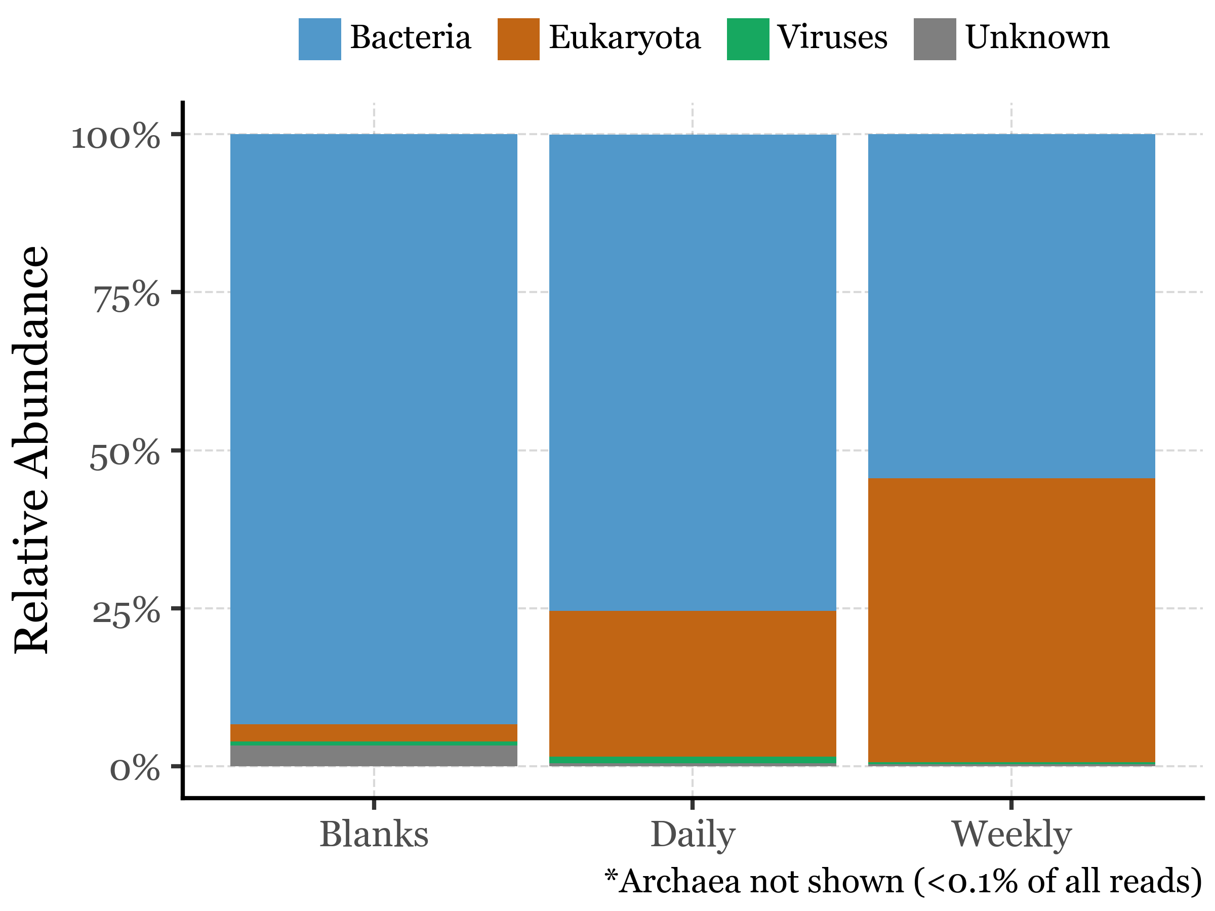
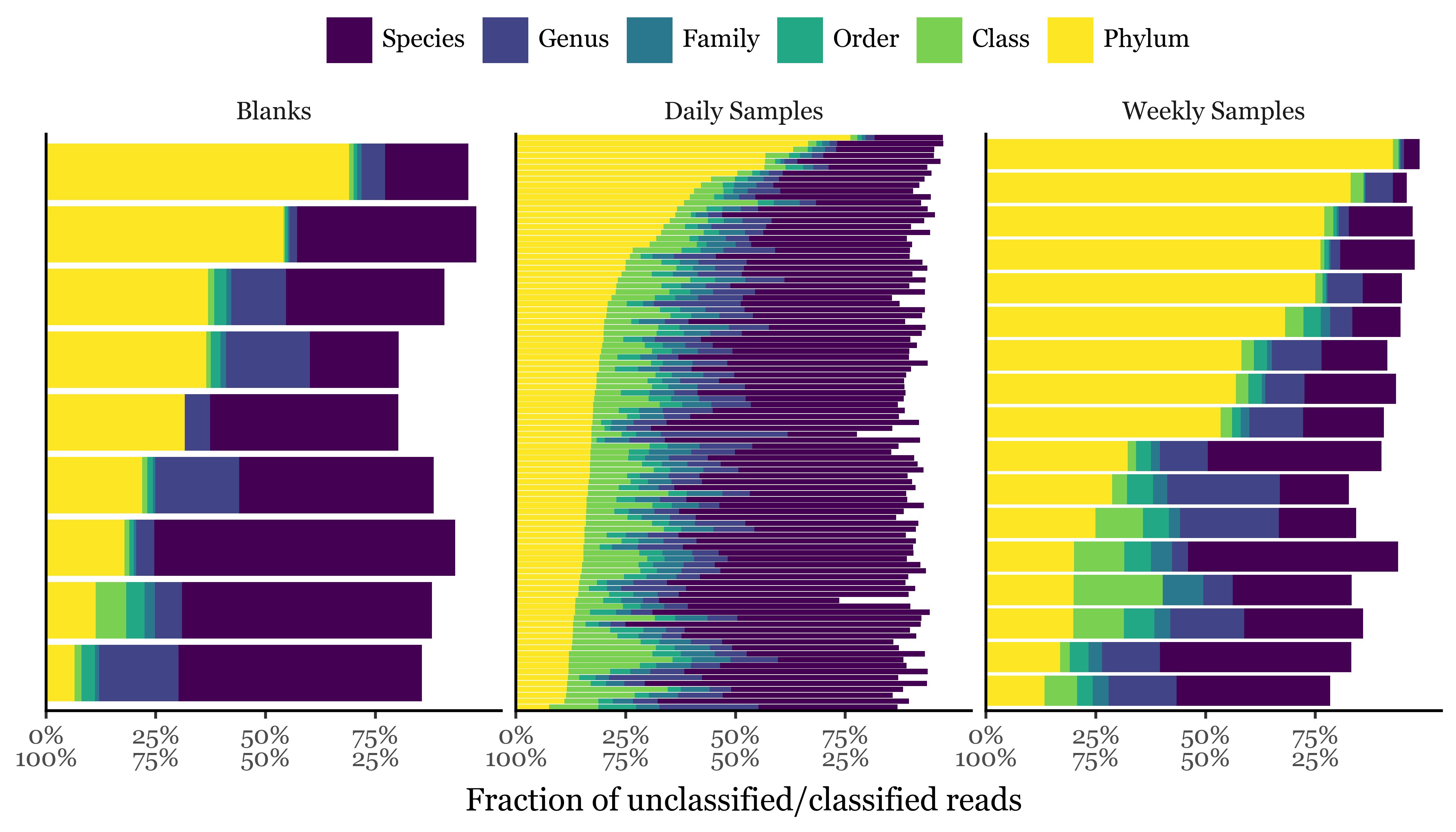
If we take a look at the assigned reads, we can see how they are distributed across different sample durations and big clades:
There seems to be a rather big contrast between the relative abundance of Bacteria and Eukaryota in the samples, with Viruses being present in much lower abundances. While the blank reads mostly belong to bacteria (93%), the daily samples show a still dominant but lower relative abundance of bacteria (75%) with respect to Eukaryota (23%). In the weekly samples, the Bacteria to Eukaryota ratio becomes much closer, however, with 54% of the reads belonging to Bacteria and 45% to Eukaryota.
Viruses are present in all samples but in very low abundances, with relative abundances ranging from 0.30 to 1.03%.
The unclassified sequences (up to this level) range from 0.35% to 0.51% in the weekly and daily samples, respectively, to 3.27% in the blanks.
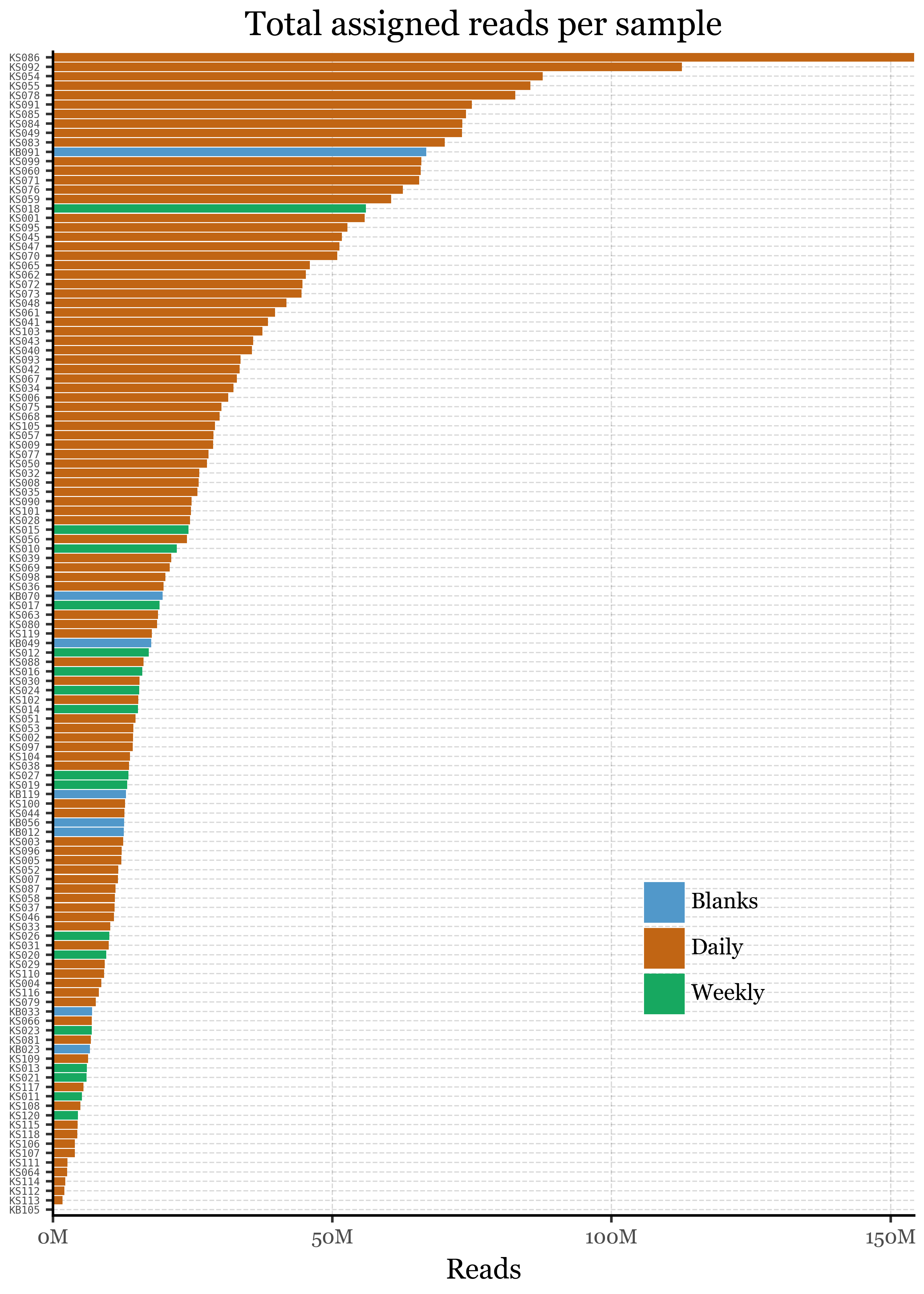
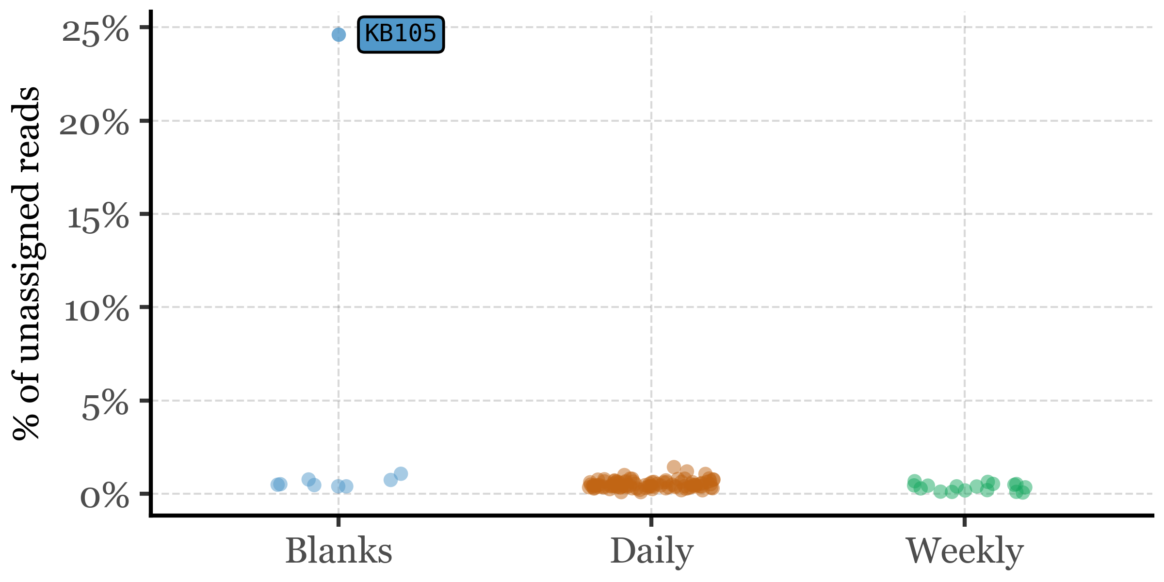
If we take a look at the percentage of unassigned reads at the big clade level per sample, however, we see how the large % of blanks is explained by a single blank sample, KB105:
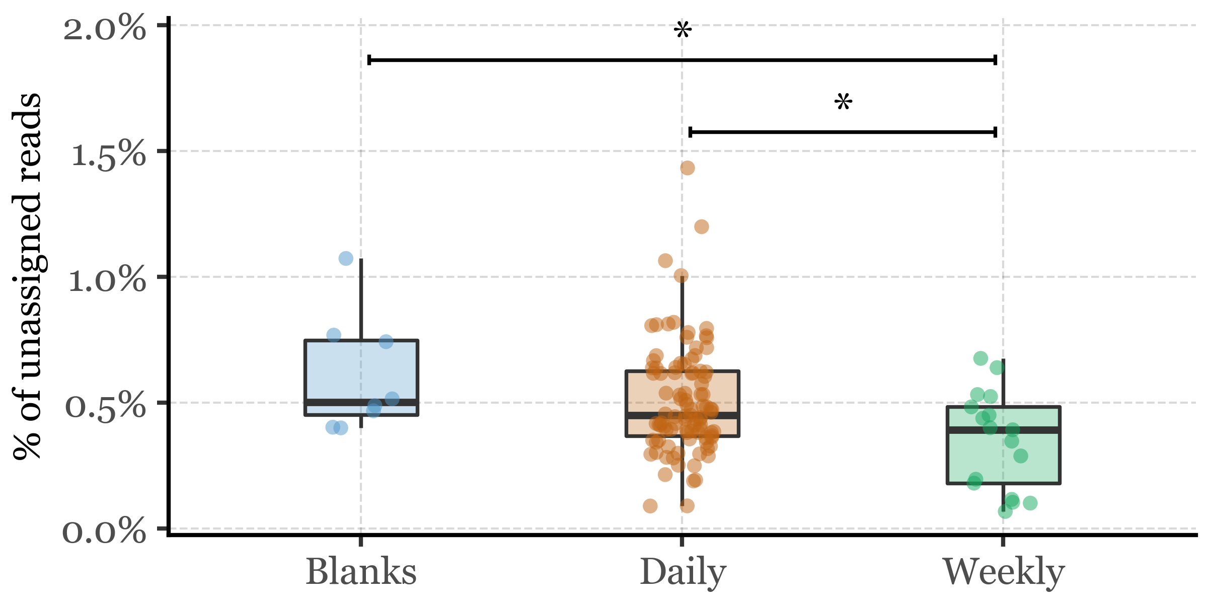
This sample is also the one with the lowest DNA yield (0.13 ng) and the lowest total read counts (roughly 100k, an order of magnitude lower than the next lowest sample that has already over a million reads) and thus it is not surprising that it has a much higher percentage of unassigned reads than the rest of the samples. Given how much of an outlier this sample is, we will remove it from the analysis and focus on the rest of the samples. If we run the comparison again between sample types, we observe that the difference in the percentage of unassigned reads persists and it’s significant between all Blanks and Weekly samples, and between Daily and Weekly samples, but not between Blanks and Daily samples:
%%R -i unassigned_datalibrary(betareg)kruskal_test <- kruskal.test(relative_abundance ~ sample_duration, data = unassigned_data)print(kruskal_test)# Dunn's test in case it's significant:if(kruskal_test$p.value <0.05) {print("Kruskal-Wallis test is significant, performing Dunn's test...") dunn_test <- FSA::dunnTest(relative_abundance ~ sample_duration, data = unassigned_data, method ="bh")print(dunn_test)}# Summary statisticssummary_stats <- unassigned_data %>% group_by(sample_duration) %>% summarise( n = n(), median = median(relative_abundance), q25 = quantile(relative_abundance, 0.25), q75 = quantile(relative_abundance, 0.75), mean = mean(relative_abundance), sd = sd(relative_abundance) )print(summary_stats)
    Kruskal-Wallis rank sum test

data:  relative_abundance by sample_duration
Kruskal-Wallis chi-squared = 7.959, df = 2, p-value = 0.0187

[1] "Kruskal-Wallis test is significant, performing Dunn's test..."
       Comparison        Z    P.unadj      P.adj
1  Blanks - Daily 1.302445 0.19276440 0.19276440
2 Blanks - Weekly 2.558239 0.01052037 0.03156111
3  Daily - Weekly 2.349434 0.01880199 0.02820298
# A tibble: 3 × 7
  sample_duration     n  median     q25     q75    mean      sd
  <chr>           <int>   <dbl>   <dbl>   <dbl>   <dbl>   <dbl>
1 Blanks              8 0.00502 0.00451 0.00749 0.00607 0.00235
2 Daily              97 0.00450 0.00369 0.00625 0.00507 0.00220
3 Weekly             17 0.00392 0.00180 0.00483 0.00349 0.00195
Dunn (1964) Kruskal-Wallis multiple comparison
  p-values adjusted with the Benjamini-Hochberg method.

Además: Aviso:
sample_duration was coerced to a factor.
Bacterial community composition
Let’s now take a look at the bacterial fraction of the taxonomic assignments for our samples. Checking out the levels of classification provided by the pipeline it seems that, roughly, the levels of classification match the following columns (which we can use to map the levels of classification to the actual names):
Since we also have plenty of reads that are assigned to names like “unclassified Bacteria” or “unclassified Micrococcus”, we will try to clean up the data and unify the names of the missing taxa or those with names that imply a lack of classification so that we can have a more consistent and informative analysis of the bacterial community composition.
Bacterial species-level abundances and species name cleaning code
# Patterns which might look like species but are too vague to be useful and shall be considered "Unclassified"bacterial_taxonomy = (taxonomy_with_ids .query('domain == "Bacteria"'))non_specific_patterns = [r'^\s*uncultured\b.*',r'^\s*unclassified\b.*',r'^\s*environmental\b.*',r'^\s*unidentified\b.*',r'^\s*bacterium\s*$', # exactly "bacterium"r'^(?:[A-Za-z]+aceae|[A-Za-z]+ales|[A-Za-z]+ia)\s+bacterium$', # Family/Order/Class + bacterium (no strain)r'^(?:marine|soil)\s+bacterium$', # marine/soil bacterium (no strain)r'^\s*cyanobacterium\s*$', # exactly "cyanobacterium"r'^[A-Z][a-z]+\s+sp\.\s*$', # Genus sp. (no strain) # any line that ends with bacterium/cyanobacterium and has no trailing strain tokenr'^(?:(?!\s+(?:bacterium|cyanobacterium)\s+[A-Za-z0-9_-]+$).)*(?:^|\s)(?:bacterium|cyanobacterium)\s*$',]def standardize_unclassified_species(name):""" If the species name matches any of the non-specific patterns, return "Unclassified" """for pattern in non_specific_patterns:if re.match(pattern, name, re.IGNORECASE):return"Unclassified"return namebacterial_abundances_long = (abundance_tax_long .merge(taxonomy_with_ids) .query('domain=="Bacteria"') .assign(species=lambda dd: np.where(dd['species'].notna(), dd['species'], np.where(dd['best_taxonomy_level'] =='strain', dd['best_taxonomy_name'].str.split(' ').str[:2].str.join(' '), np.where(dd['best_taxonomy_level'] =='subspecies', dd['best_taxonomy_name'].str.split(' ').str[:2].str.join(' '), "Unclassified"))))# if species matches any of the non-specific patterns, set to "Unclassified"# .assign(species=lambda dd: dd['species'].apply(standardize_unclassified_species)) .groupby(['domain', 'phylum', 'class', 'order', 'family', 'genus', 'species', 'best_taxonomy_level'] + ['sample_id'], as_index=False, dropna=False) .agg(counts=('counts', 'sum')))
---------------------------------------------------------------------------NameError Traceback (most recent call last)
CellIn[116], line 6 1#| code-fold: true 2#| code-summary: Bacterial species-level abundances and species name cleaning code 3 4# Patterns which might look like species but are too vague to be useful and shall be considered "Unclassified"----> 6 bacterial_taxonomy = (taxonomy_with_ids 7 .query('domain == "Bacteria"')
8 )
9 non_specific_patterns = [
10r'^\s*uncultured\b.*',
11r'^\s*unclassified\b.*',
(...) 20r'^(?:(?!\s+(?:bacterium|cyanobacterium)\s+[A-Za-z0-9_-]+$).)*(?:^|\s)(?:bacterium|cyanobacterium)\s*$',
21 ]
23defstandardize_unclassified_species(name):
NameError: name 'taxonomy_with_ids' is not defined
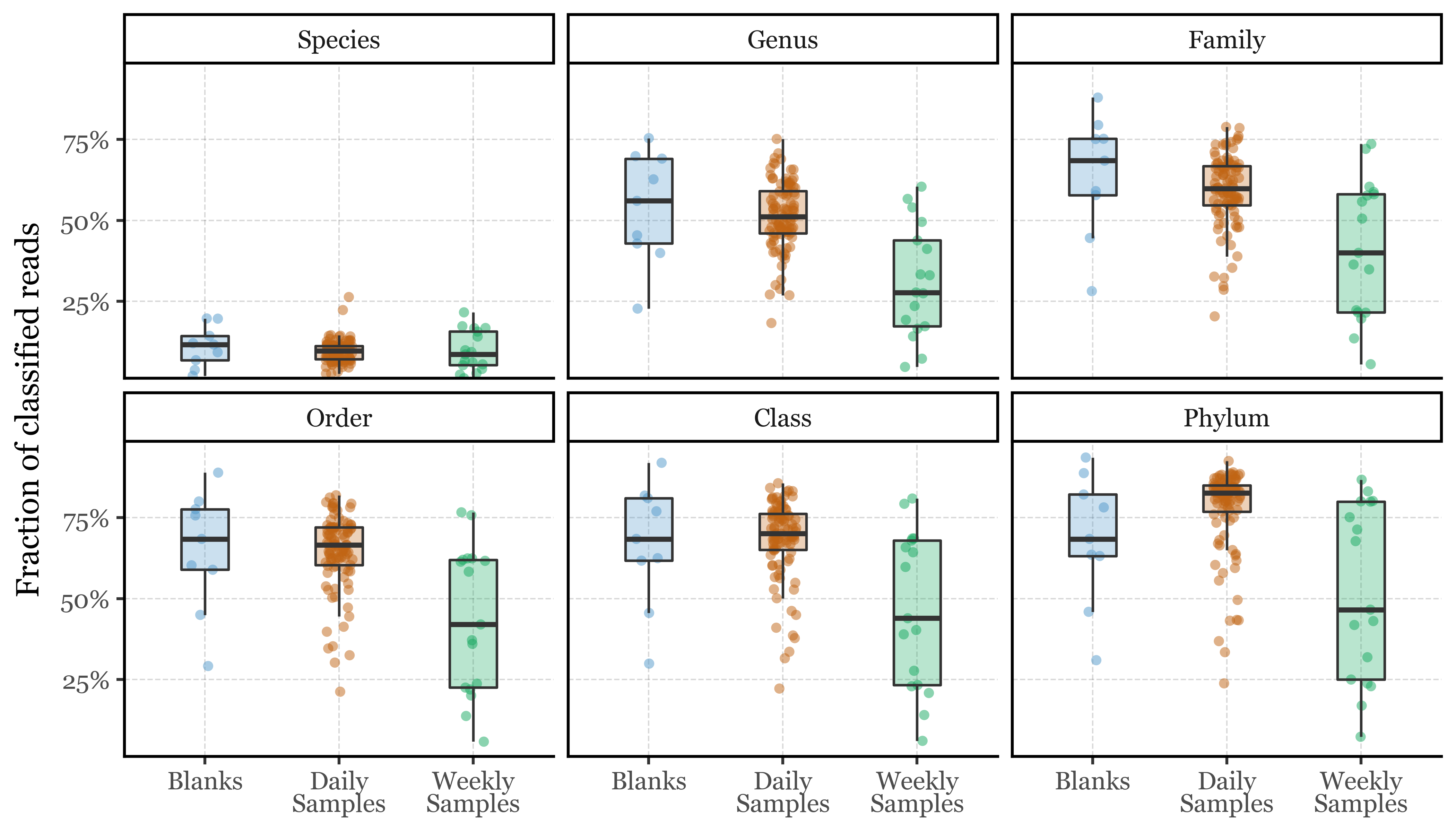
Meaning that, for Species, we have an average of around 11% of all reads classified at this level (and thus, 89% unclassified), quite consistently across all sample types. The boxplots below show the comparison for each of these levels, with the table summarizing the average percentage of assigned reads at each level. Strikingly, the weekly samples have the lowest percentage of assigned reads at all taxonomic levels, with a sizable chunk of weekly samples having a pretty low % of assigned reads even at the Phylum level, which is quite concerning and might indicate that degradation of bacterial DNA is happening at a quite high rate in these samples.
(unclassified_reads_df .assign(classified_rate=lambda dd: 1- dd['unclassified_rate']) .groupby(['sample_duration', 'taxonomy_level']).agg({'classified_rate': 'mean',}).reset_index().rename(columns={'sample_duration': 'Sample Group'}).pivot(index='taxonomy_level', columns='Sample Group', values='classified_rate').style.format('{:.2%}').set_caption("Average fraction of classified reads per taxonomic level"))
Table 1: Average fraction of classified reads per taxonomic level
Sample Group
Blanks
Daily Samples
Weekly Samples
taxonomy_level
Species
11.06%
9.59%
9.68%
Genus
53.76%
51.51%
31.19%
Family
63.95%
59.04%
41.31%
Order
64.87%
64.42%
43.74%
Class
66.64%
68.25%
46.66%
Phylum
68.28%
77.55%
51.97%
Now, the total number of reads which end up unassigned at the Species and Genus level is really high, with way over 50% of all reads not even assigned to a Genus, and over 90% not assigned to a Species.
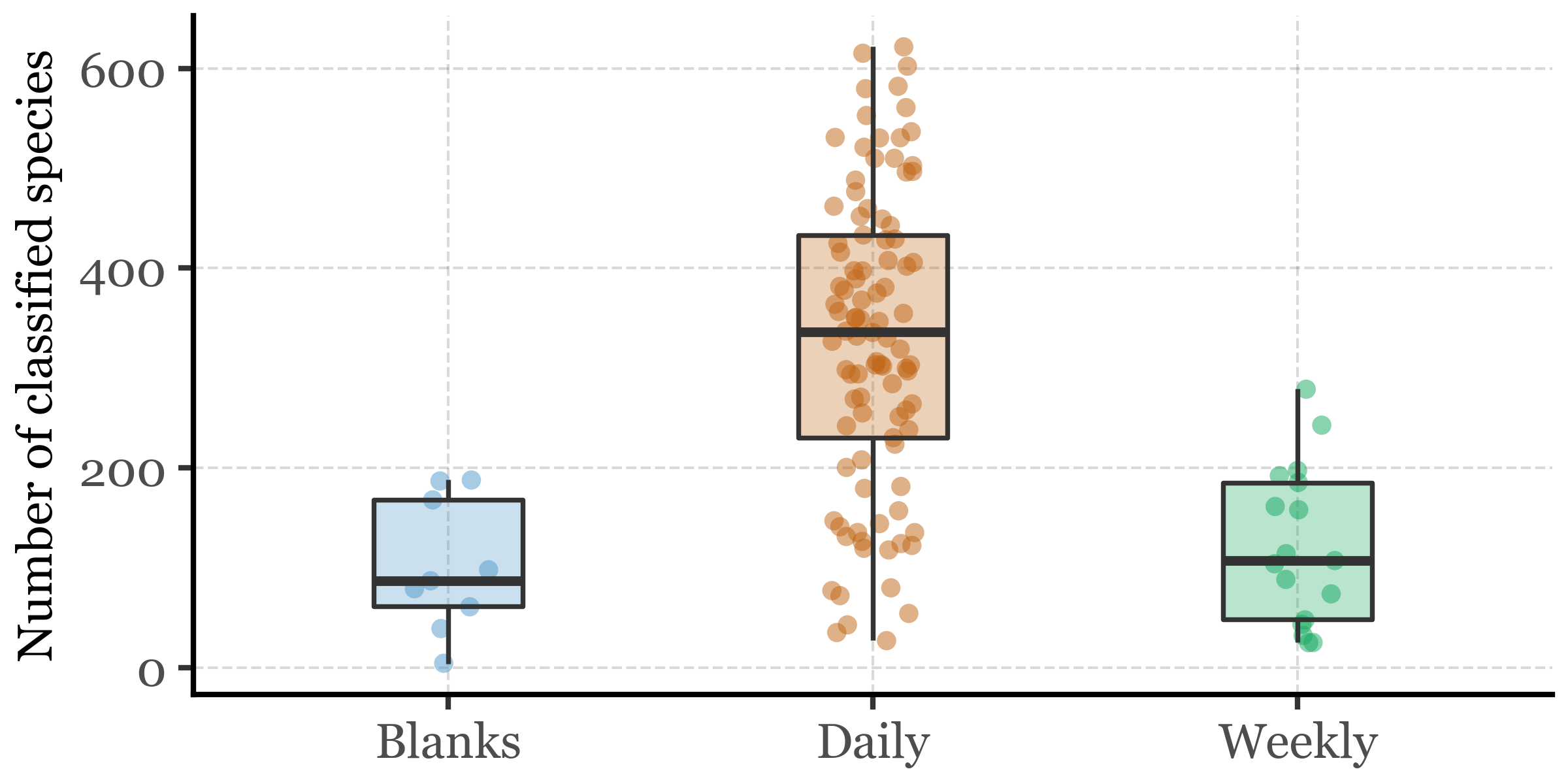
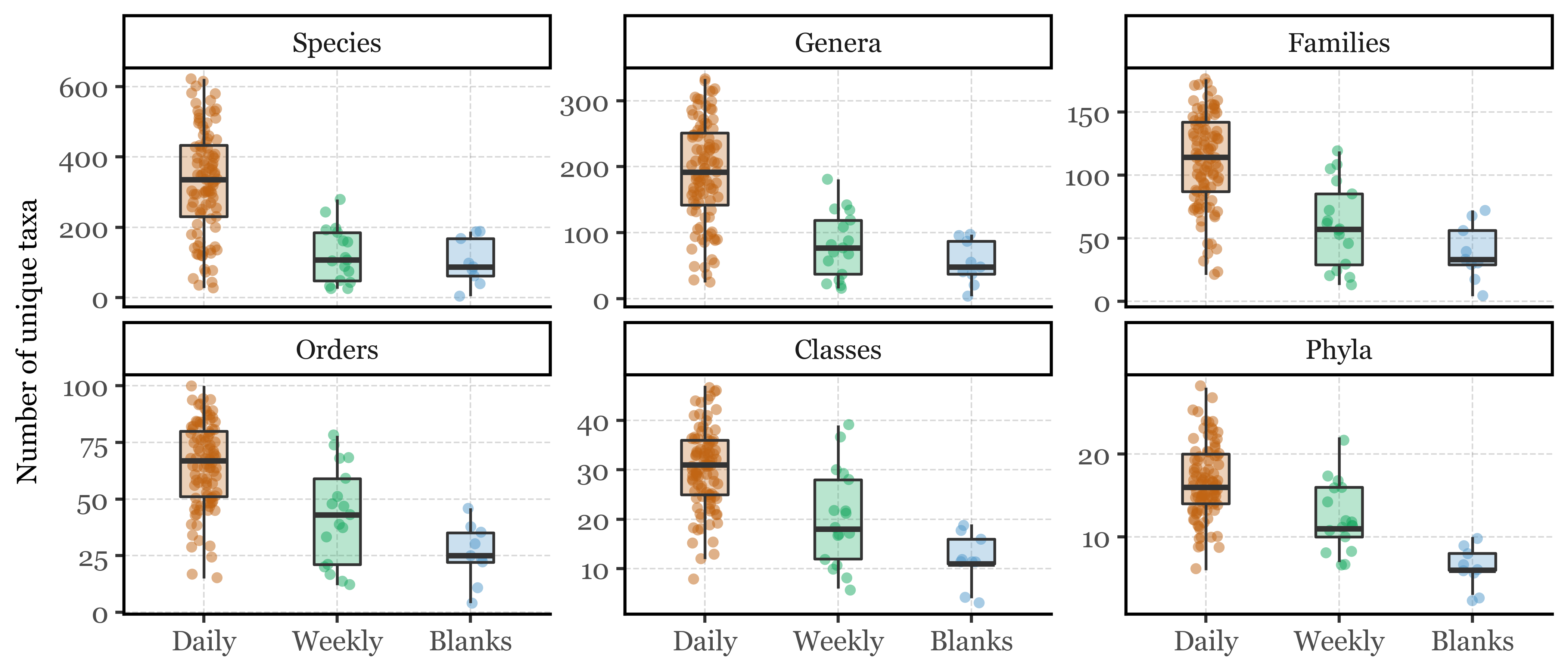
However, in absolute terms, this low fraction still provides us with a rich abundance of information about a rich diversity of Bacteria. Let’s put that into numbers:
Table of mean number of unique bacterial species per sample group
(bacterial_abundances_long .query('counts > 0') .query('species != "Unclassified"') .groupby(['sample_id'], as_index=False) .species.nunique() .merge(kumamoto_metadata[['sample_id', 'sample_duration']], how='left', on='sample_id') .groupby('sample_duration', as_index=False) .agg({'species': 'mean'}) .rename(columns={'species': 'Mean n of unique species','sample_duration': 'Sample Group'}) .style .hide(axis='index') .format({'Mean n of unique species': '{:.1f}' }))
Sample Group
Mean n of unique species
Blanks
101.2
Daily
329.1
Weekly
122.1
Table of mean number of unique bacterial genus per sample group
(genus_abundances .groupby('sample_id') .agg({'genus': 'nunique'}) .merge(kumamoto_metadata[['sample_id', 'sample_duration']], how='left', on='sample_id') .groupby('sample_duration', as_index=False) .agg({'genus': 'mean'}) .rename(columns={'genus': 'Mean n of unique genera','sample_duration': 'Sample Group'}) .style .hide(axis='index') .format({'Mean n of unique genera': '{:.1f}'}))
Sample Group
Mean n of unique genera
Blanks
77.8
Daily
264.5
Weekly
115.9
Show Code
# We will create a sample x genus table for later usebacterial_genus_table = (bacterial_abundances_long .query('counts > 0') .query('genus.notna() & genus != "Unclassified"') .groupby(['sample_id', 'genus'])['counts'] .sum() .pivot(index='sample_id', columns='genus', values='counts'))
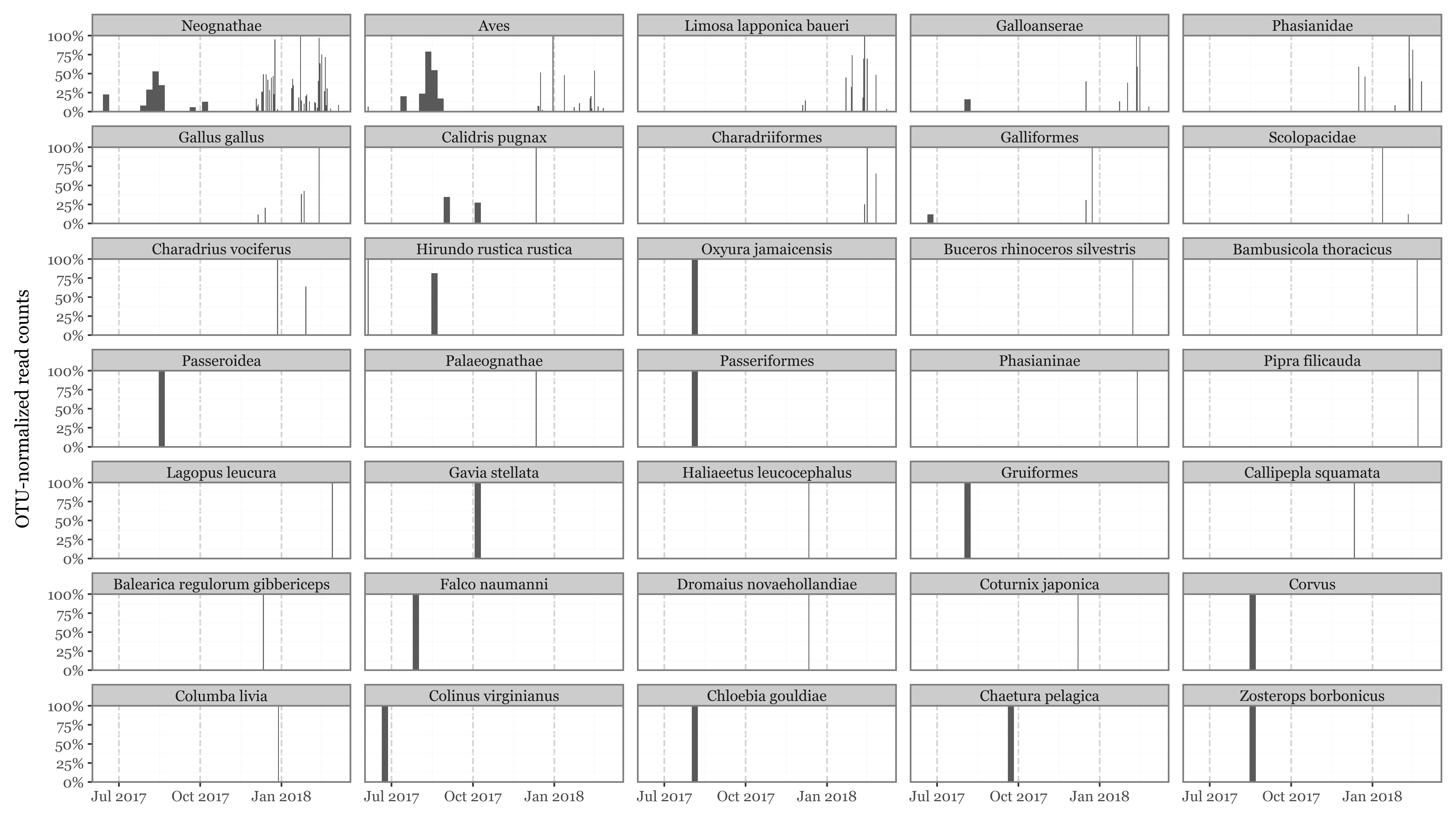
aves_notes = {"Neognathae": "Clade containing most modern birds except ratites and tinamous.","Palaeognathae": "Clade including ratites (ostrich, emu) and tinamous.","Limosa lapponica baueri": "Bar-tailed godwit subspecies, a long-distance migratory shorebird.","Aves": "Class of all birds.","Phasianidae": "Family of ground-dwelling birds including pheasants, chickens, and turkeys.","Gallus gallus": "Red junglefowl, wild ancestor of domestic chickens.","Calidris pugnax": "Ruff, a migratory wader species in the sandpiper family.","Scolopacidae": "Family of wading birds like sandpipers and curlews.","Galloanserae": "Clade grouping landfowl (Galliformes) and waterfowl (Anseriformes).","Charadrius vociferus": "Killdeer, a plover common in open habitats in North America.","Haliaeetus leucocephalus": "Bald eagle, large bird of prey from North America.","Hirundo rustica rustica": "Nominate subspecies of barn swallow, widespread in Eurasia.","Charadriiformes": "Order of shorebirds including plovers, gulls, and auks.","Colinus virginianus": "Northern bobwhite, a quail native to North America.","Pipra filicauda": "Wire-tailed manakin, a small South American bird.","Galliformes": "Order of heavy-bodied ground-feeding birds (chickens, turkeys, quails).","Columba livia": "Rock pigeon, common in urban areas worldwide.","Coturnix japonica": "Japanese quail, a domesticated quail species.","Dromaius novaehollandiae": "Emu, large flightless bird native to Australia.","Phasianinae": "Subfamily of pheasants and related birds.","Balearica regulorum gibbericeps": "Grey crowned crane subspecies from Africa.","Chloebia gouldiae": "Gouldian finch, a colorful Australian passerine.","Bambusicola thoracicus": "Chinese bamboo partridge, a ground bird from East Asia.","Gruiformes": "Order including cranes, rails, and coots.","Buceros rhinoceros silvestris": "Subspecies of rhinoceros hornbill from Southeast Asia.","Oxyura jamaicensis": "Ruddy duck, a stiff-tailed duck from the Americas.","Chaetura pelagica": "Chimney swift, a migratory bird from the Americas.","Falco naumanni": "Lesser kestrel, a small migratory falcon.","Callipepla squamata": "Scaled quail, found in southwestern US and Mexico.","Zosterops borbonicus": "Réunion grey white-eye, endemic passerine to Réunion Island.","Gavia stellata": "Red-throated loon, a migratory aquatic bird.","Passeroidea": "Superfamily of passerine birds including sparrows and finches.","Corvus": "Genus of crows, ravens, rooks, and jackdaws.","Lagopus leucura": "White-tailed ptarmigan, a grouse living in alpine habitats.","Passeriformes": "Order of perching birds, the largest bird order."}aves_unlikely_presence = ["Dromaius novaehollandiae", "Chloebia gouldiae", "Buceros rhinoceros silvestris", "Haliaeetus leucocephalus","Balearica regulorum gibbericeps","Pipra filicauda",](abundance_tax_long .query('level_27 == " Aves"') .assign(full_name=lambda dd: dd.apply(lambda row: '; '.join(row[tax_levels].dropna()), axis=1)) .assign(last_name=lambda dd: dd.full_name.str.split(';').str[-1].str.strip()) .groupby('last_name', as_index=False) .agg({'counts': 'sum'}) .sort_values('counts', ascending=False) .assign(Frequency=lambda dd: dd.counts / dd.counts.sum()) .assign(note=lambda dd: dd.last_name.map(aves_notes).fillna('')) .rename(columns={'last_name': 'Name (deepest tax. level)','counts': 'Reads'}) .style .format({'Frequency': '{:.2%}','Reads': '{:.0f}'}) .hide(axis='index')# text align left .set_properties(**{'text-align': 'left', 'font-family': 'monospace','font-size': '9pt','width' : '1200 px'}) .bar(subset=['Frequency'], color='#5198ca', align='mid')# color red for unlikely presence .map(lambda x: 'color: red'if x in aves_unlikely_presence else'color: none', subset=['Name (deepest tax. level)'] ))
Name (deepest tax. level)
Reads
Frequency
note
Neognathae
253914
40.23%
Clade containing most modern birds except ratites and tinamous.
Limosa lapponica baueri
113472
17.98%
Bar-tailed godwit subspecies, a long-distance migratory shorebird.
Aves
59533
9.43%
Class of all birds.
Phasianidae
39584
6.27%
Family of ground-dwelling birds including pheasants, chickens, and turkeys.
Gallus gallus
33016
5.23%
Red junglefowl, wild ancestor of domestic chickens.
Calidris pugnax
16638
2.64%
Ruff, a migratory wader species in the sandpiper family.
Scolopacidae
9934
1.57%
Family of wading birds like sandpipers and curlews.
Galloanserae
9279
1.47%
Clade grouping landfowl (Galliformes) and waterfowl (Anseriformes).
Charadrius vociferus
9086
1.44%
Killdeer, a plover common in open habitats in North America.
Haliaeetus leucocephalus
8342
1.32%
Bald eagle, large bird of prey from North America.
Hirundo rustica rustica
7571
1.20%
Nominate subspecies of barn swallow, widespread in Eurasia.
Charadriiformes
7351
1.16%
Order of shorebirds including plovers, gulls, and auks.
Colinus virginianus
6431
1.02%
Northern bobwhite, a quail native to North America.
Pipra filicauda
4862
0.77%
Wire-tailed manakin, a small South American bird.
Galliformes
4575
0.72%
Order of heavy-bodied ground-feeding birds (chickens, turkeys, quails).
Columba livia
4470
0.71%
Rock pigeon, common in urban areas worldwide.
Coturnix japonica
3955
0.63%
Japanese quail, a domesticated quail species.
Dromaius novaehollandiae
3812
0.60%
Emu, large flightless bird native to Australia.
Phasianinae
3453
0.55%
Subfamily of pheasants and related birds.
Balearica regulorum gibbericeps
3222
0.51%
Grey crowned crane subspecies from Africa.
Chloebia gouldiae
3059
0.48%
Gouldian finch, a colorful Australian passerine.
Bambusicola thoracicus
2705
0.43%
Chinese bamboo partridge, a ground bird from East Asia.
Gruiformes
2646
0.42%
Order including cranes, rails, and coots.
Buceros rhinoceros silvestris
2409
0.38%
Subspecies of rhinoceros hornbill from Southeast Asia.
Oxyura jamaicensis
2274
0.36%
Ruddy duck, a stiff-tailed duck from the Americas.
Chaetura pelagica
2236
0.35%
Chimney swift, a migratory bird from the Americas.
Falco naumanni
2210
0.35%
Lesser kestrel, a small migratory falcon.
Callipepla squamata
2168
0.34%
Scaled quail, found in southwestern US and Mexico.
Zosterops borbonicus
1963
0.31%
Réunion grey white-eye, endemic passerine to Réunion Island.
Gavia stellata
1959
0.31%
Red-throated loon, a migratory aquatic bird.
Passeroidea
1683
0.27%
Superfamily of passerine birds including sparrows and finches.
Corvus
1469
0.23%
Genus of crows, ravens, rooks, and jackdaws.
Lagopus leucura
942
0.15%
White-tailed ptarmigan, a grouse living in alpine habitats.
Palaeognathae
663
0.11%
Clade including ratites (ostrich, emu) and tinamous.