import numpy as np
import pandas as pd
import plotnine as p9
import matplotlib.pyplot as plt

from matplotlib_inline.backend_inline import set_matplotlib_formatsNoto Subdaily Samples
Preamble
Show code imports and presets
Imports
Pre-sets
# Matplotlib settings
plt.rcParams['font.family'] = 'Georgia'
set_matplotlib_formats('retina')

# Plotnine settings (for figures)

p9.options.set_option('base_family', 'Georgia')

p9.theme_set(
    p9.theme_bw()
    + p9.theme(panel_border=p9.element_rect(size=2),
               panel_grid=p9.element_blank(),
               axis_ticks_major=p9.element_line(size=2, markersize=3),
               axis_text=p9.element_text(size=11),
               axis_title=p9.element_text(size=14),
               plot_title=p9.element_text(size=17),
               legend_background=p9.element_blank(),
               legend_text=p9.element_text(size=12),
               strip_text=p9.element_text(size=13),
               strip_background=p9.element_rect(size=2),
               panel_grid_major=p9.element_line(size=1, linetype='dashed',
                                                alpha=.15, color='black'),
    )
)
Reading Data
taxons = ['Kingdom', 'Phylum', 'Class', 'Order', 'Family', 'Genus', 'Species']subdaily_metals = pd.read_excel('../data/NOTO_FINAL.xlsx', sheet_name=2, index_col=1)samples_info = (pd.read_excel('../data/Filters_inventory.xlsx',
sheet_name='Noto_2015_2016', skiprows=5)
.iloc[:, list(range(4)) + [7]]
.rename(columns={'Unnamed: 0': 'sample_id'})
.loc[lambda dd: dd.sample_id.notna()]
.ffill()
.loc[lambda dd: dd.sample_id.str.startswith('S')]
.assign(initial=lambda dd: pd.to_datetime(dd.Date.astype(str) +
' ' + dd.Initial.astype(str)))
.assign(final=lambda dd: pd.to_datetime(dd.Date.astype(str) +
' ' + dd.Final.astype(str)))
.assign(final=lambda dd:
np.where(dd.final.dt.hour < 9, dd.final + pd.Timedelta('1 day'), dd.final))
.assign(hours_sampled=lambda dd: (dd.final - dd.initial)
.apply(lambda x: pd.Timedelta(x).seconds / 3600))
.rename(columns={'Sampled air volume (m3)': 'sampled_volume'})
[['sample_id', 'initial', 'final', 'sampled_volume', 'hours_sampled']]
.reset_index(drop=True)
)
samples_info.set_index('sample_id')| initial | final | sampled_volume | hours_sampled | |
|---|---|---|---|---|
| sample_id | ||||
| S46 | 2015-02-23 12:30:00 | 2015-02-23 14:30:00 | 60.0 | 2.000000 |
| S47 | 2015-02-23 15:30:00 | 2015-02-23 17:30:00 | 60.1 | 2.000000 |
| S48 | 2015-02-23 18:35:00 | 2015-02-24 08:30:00 | 417.7 | 13.916667 |
| S49 | 2015-02-24 09:30:00 | 2015-02-24 11:30:00 | 60.0 | 2.000000 |
| S50 | 2015-02-24 12:30:00 | 2015-02-24 14:30:00 | 60.0 | 2.000000 |
| S51 | 2015-02-24 15:30:00 | 2015-02-24 17:30:00 | 60.0 | 2.000000 |
| S52 | 2015-02-24 18:30:00 | 2015-02-25 08:30:00 | 419.7 | 14.000000 |
| S53 | 2015-02-25 09:35:00 | 2015-02-25 11:35:00 | 60.0 | 2.000000 |
| S54 | 2015-02-25 12:30:00 | 2015-02-25 14:30:00 | 60.1 | 2.000000 |
| S55 | 2015-02-25 15:30:00 | 2015-02-25 17:30:00 | 60.0 | 2.000000 |
| S56 | 2015-02-25 18:30:00 | 2015-02-26 08:30:00 | 419.6 | 14.000000 |
| S57 | 2015-02-26 09:34:00 | 2015-02-26 11:34:00 | 60.0 | 2.000000 |
| S58 | 2015-02-26 12:30:00 | 2015-02-26 14:30:00 | 59.9 | 2.000000 |
| S59 | 2015-02-26 15:30:00 | 2015-02-26 17:30:00 | 60.1 | 2.000000 |
| S60 | 2015-02-26 18:30:00 | 2015-02-27 08:30:00 | 419.0 | 14.000000 |
| S61 | 2015-02-27 09:30:00 | 2015-02-27 11:30:00 | 60.1 | 2.000000 |
| S62 | 2015-02-27 12:35:00 | 2015-02-27 14:35:00 | 60.0 | 2.000000 |
| S63 | 2015-02-27 15:30:00 | 2015-02-27 17:30:00 | 60.0 | 2.000000 |
| S64 | 2015-02-27 18:30:00 | 2015-02-28 08:30:00 | 419.0 | 14.000000 |
subdaily_samples = (pd.concat([pd.read_excel('../data/NOTO_FINAL.xlsx', sheet_name='16S Noto'),
pd.read_excel('../data/NOTO_FINAL.xlsx', sheet_name='ITS Noto')])
.loc[lambda dd: dd.Kingdom.notna()]
.loc[:, lambda dd: [(x in samples_info.sample_id.unique() or x in taxons) for x in dd.columns]]
.apply(lambda x: x.str.split('__').str[-1] if x.name in taxons else x)
.fillna({t: 'unknown' for t in taxons}) # fill partially identified taxa with unknown
.fillna(0) # 0-fill missing values
.melt(taxons, var_name='sample_id', value_name='abundance')
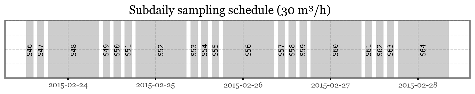
)(p9.ggplot(samples_info)
+ p9.geom_rect(mapping=p9.aes(xmin='initial', xmax='final'), ymin=0, ymax=1, alpha=.3)
+ p9.geom_text(p9.aes(x='initial + (final - initial) / 2', label='sample_id', y=.5),
angle=90, family='monospace', size=10)
+ p9.theme(figure_size=(12, 1.5),
axis_text_y=p9.element_blank(),
axis_ticks_major_y=p9.element_blank(),
axis_ticks_minor_y=p9.element_blank())
+ p9.labs(x='', y='', title='Subdaily sampling schedule (30 m³/h)')
)
Metagenomics
While most filters collected data for a total of 2 hours, samples 48, 52, 56, 60 and 64 were sampling overnight, for a total of 14 hours each. The sampling volume was of 30 m³/h in all cases.
As far as my knowledge goes, there is no normalization of the sequence counts based on the total volume sampled, so unless we are reaching the limit of capacity of the filters or somehow the samples start to degrade after a certain amount time, we would expect to find more total sequence counts in those filters that sampled a higher volume.
Of course, it is not that simple, because the total airborne microbial mass is not constant during the whole day, and follows daily cycles. Since the higher volume samples were all taken during the nights, a lower nightly microbial mass could lead to a decreased number of sequence counts during the longer nightly samples. Taking into account the sampled volume is 7x the one during daily samples, the difference should be really drastic to not see an increase in the number of total counts in those samples. Let’s see the raw results:
(subdaily_samples
 .loc[lambda dd: dd.Kingdom.isin(['Bacteria', 'Fungi'])]
 .groupby(['Kingdom', 'sample_id'], as_index=False)
 .abundance.sum()
 .pipe(lambda dd: p9.ggplot(dd)
       + p9.aes('sample_id', 'abundance', fill='Kingdom')
       + p9.geom_col(position='dodge')
       + p9.theme_bw()
       + p9.theme(figure_size=(8, 1.5))
       + p9.labs(x='Sample ID', y='Sequence Counts'))
)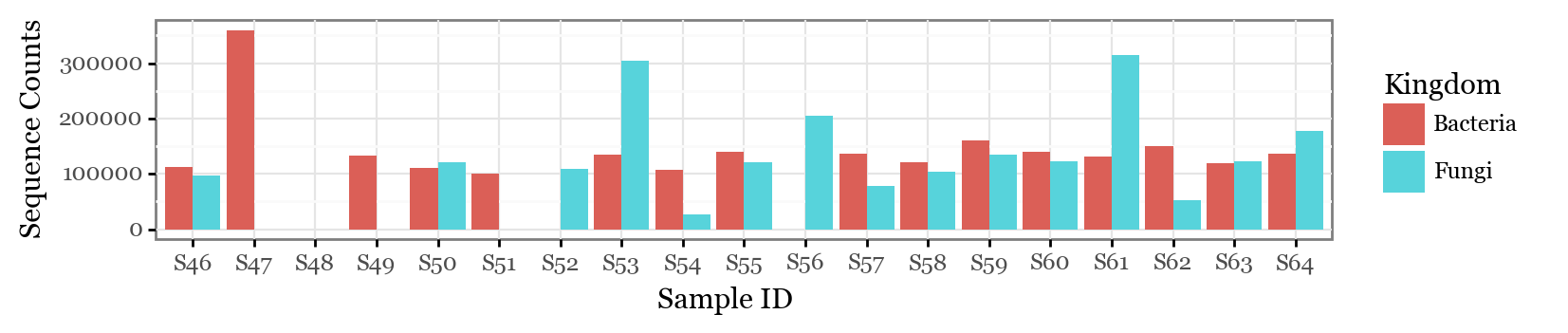
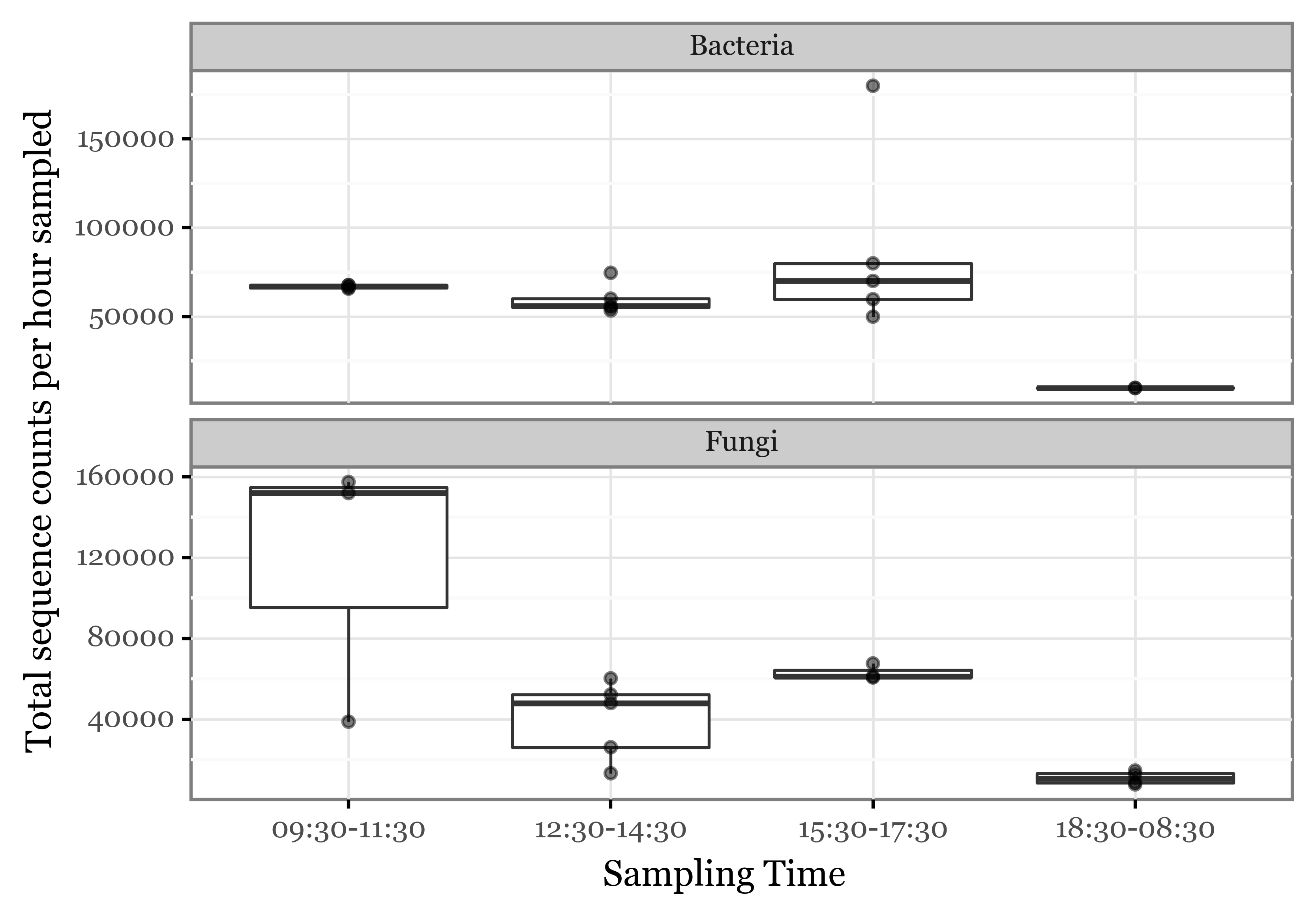
In several samples, we could not recover either the bacterial or the fungal fraction. In sample 48, neither of them. However, what we can see is that there is not an apparent increase in sequence counts during the long nigthly samples for either of bacterial or fungal sequences. If we go further and look at the total counts per hour sampled, the differences are even more drastic:
(subdaily_samples
 .loc[lambda dd: dd.Kingdom.isin(['Bacteria', 'Fungi'])]
 .groupby(['sample_id', 'Kingdom'], as_index=False)
 .abundance.sum()
 .merge(samples_info)
 .assign(counts_per_h=lambda dd: dd.abundance / dd.hours_sampled)
 .pipe(lambda dd: p9.ggplot(dd)
       + p9.geom_rect(mapping=p9.aes(xmin='initial', xmax='final', ymax='counts_per_h'), ymin=0, alpha=.3)
       + p9.geom_text(p9.aes(label='sample_id', x='initial + (final - initial) / 2'),
                      angle=90, y=dd.counts_per_h.max() / 10, family='monospace', size=9)
       + p9.theme_bw()
       + p9.theme(figure_size=(10, 4))
       + p9.facet_wrap('Kingdom', ncol=1)
       + p9.labs(x='Date', y='Sequence counts per hour sampled', title='Subdaily sampling time overview'))
)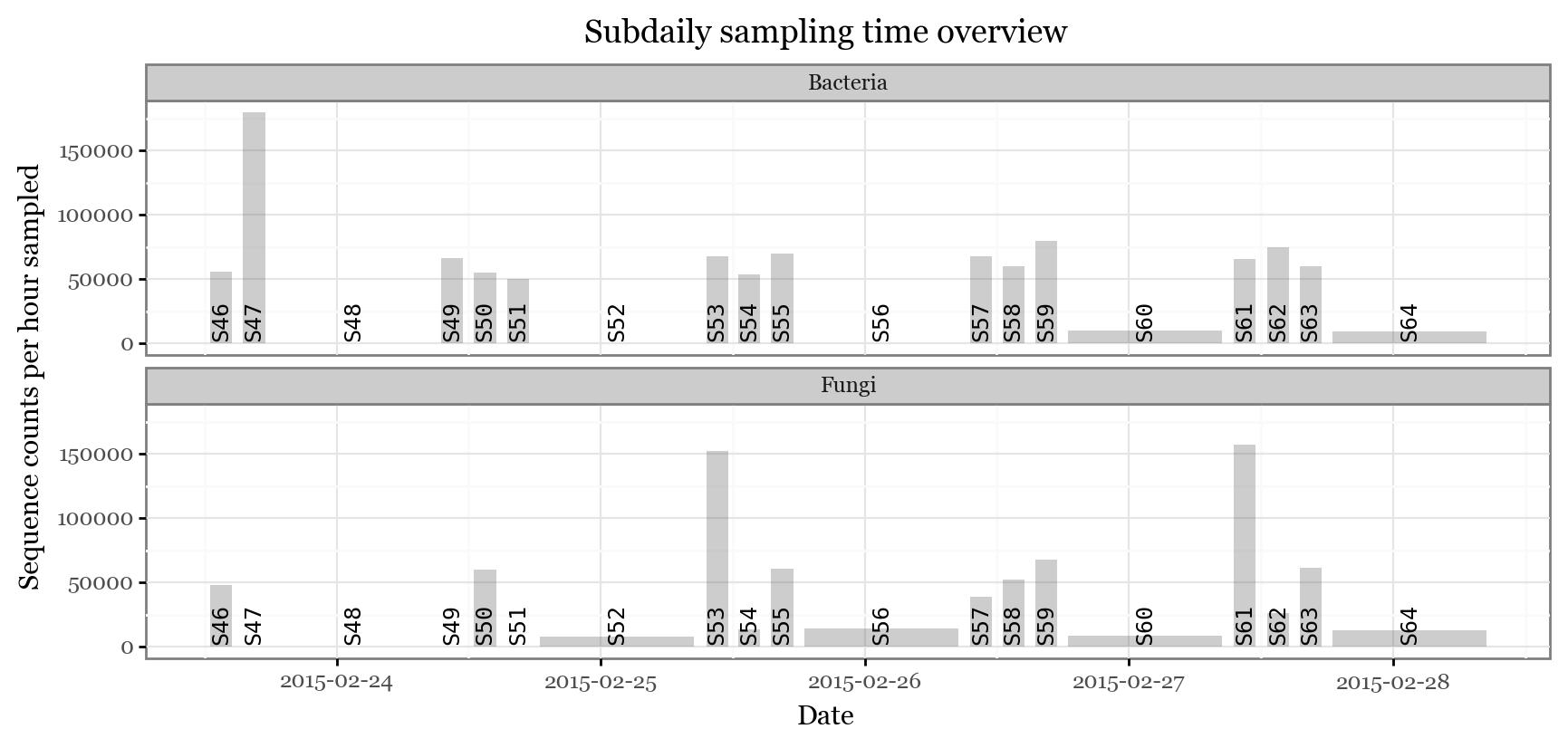
While it is possible we might have hit the limit of viable hours the filters can keep consistently microbial biomass with recoverable DNA, it is also likely that the nightly yield per hour is simply lower.
In [1], they take 12 2h daily samples for several days in Singapore. While in different conditions, they observe that: + The diversity of the samples peaks around noon and is much higher during the day than during the night:

- The DNA yield, however, was found to fluctuate on the opposite direction. Citing the study:
The total sampled biomass was consistently higher during night hours (19:00 to 07:00), as approximated by DNA amount extracted per 2-h interval (Fig. 4A). The DNA amounts varied between 5 and 500 ng (per 72 m³ sampled), resulting in up to a 100-fold difference between the early morning hours (05:00) and solar noon (13:00) (e.g., DVE2). This diel effect continued to exist during the dry seasons, but the DNA amount declined ∼30-fold to 5 to 150 ng (e.g., DVE3 and 4).

Let’s check the \(\alpha\)-diversity of our samples to check whether the dynamics here are similar to those in the Singapore study:
(subdaily_samples
 .loc[lambda dd: dd.abundance > 5]
 .loc[lambda dd: dd.Kingdom.isin(['Bacteria', 'Fungi'])]
 .groupby(['sample_id', 'Kingdom'])
 .size()
 .rename('n_taxa')
 .reset_index()
 .merge(samples_info)
 .pipe(lambda dd: p9.ggplot(dd)
       + p9.geom_rect(mapping=p9.aes(xmin='initial', xmax='final', ymax='n_taxa'), ymin=0, alpha=.3)
       + p9.geom_text(p9.aes(label='sample_id', x='initial + (final - initial) / 2'),
                      angle=90, y=dd.n_taxa.max() / 5, family='monospace', size=9)
       + p9.theme_bw()
       + p9.theme(figure_size=(10, 3))
       + p9.facet_wrap('Kingdom', ncol=1)
       + p9.labs(x='Date', y='Unique taxa', title=r'$\alpha$-Diversity of subdaily samples')))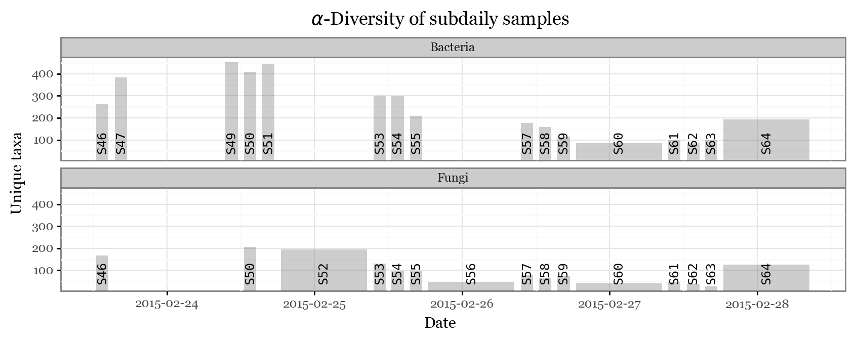
samples_info = samples_info.assign(initial=lambda dd: dd.initial.dt.round('30min'),
final=lambda dd: dd.final.dt.round('30min'),
centroid=lambda dd: dd.initial + (dd.final - dd.initial) / 2,
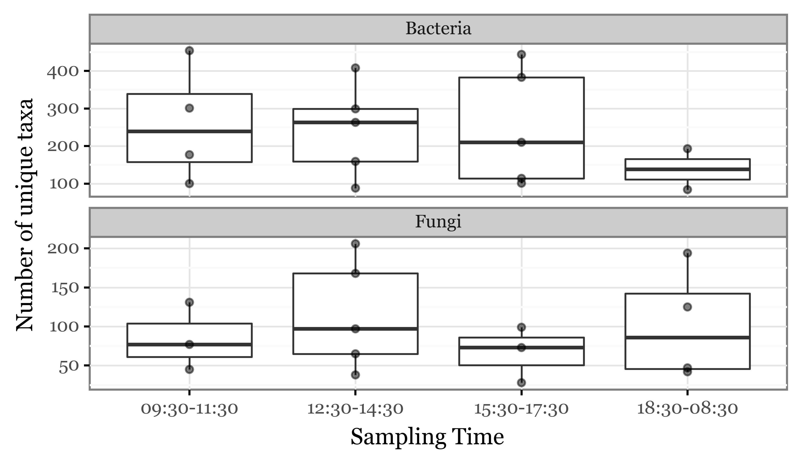
time_slot=lambda dd: dd.initial.dt.strftime('%H:%M') + '-' + dd.final.dt.strftime('%H:%M'))Diversity per time-slot
(subdaily_samples
 .loc[lambda dd: dd.abundance > 5]
 .loc[lambda dd: dd.Kingdom.isin(['Bacteria', 'Fungi'])]
 .groupby(['sample_id', 'Kingdom'])
 .size()
 .rename('n_taxa')
 .reset_index()
 .merge(samples_info)
 .pipe(lambda dd: p9.ggplot(dd)
       + p9.aes('time_slot', 'n_taxa')
       + p9.geom_boxplot(outlier_alpha=0)
       + p9.geom_point(alpha=.5)
       + p9.facet_wrap('Kingdom', scales='free_y', ncol=1)
       + p9.theme_bw()
       + p9.theme(figure_size=(6, 3), dpi=300)
       + p9.labs(x='Sampling Time', y='Number of unique taxa'))
)
Abundance per time-slot
(subdaily_samples
 .loc[lambda dd: dd.abundance > 5]
 .loc[lambda dd: dd.Kingdom.isin(['Bacteria', 'Fungi'])]
 .groupby(['sample_id', 'Kingdom'])
 .abundance.sum()
 .reset_index()
 .merge(samples_info)
 .pipe(lambda dd: p9.ggplot(dd)
       + p9.aes('time_slot', 'abundance')
       + p9.geom_boxplot(outlier_alpha=0)
       + p9.geom_point(alpha=.5)
       + p9.facet_wrap('Kingdom', scales='free_y', ncol=1)
       + p9.theme_bw()
       + p9.theme(dpi=300, figure_size=(6, 4))
       + p9.labs(x='Sampling Time', y='Total sequence counts'))
)
(subdaily_samples
 .loc[lambda dd: dd.abundance > 5]
 .loc[lambda dd: dd.Kingdom.isin(['Bacteria', 'Fungi'])]
 .groupby(['sample_id', 'Kingdom'])
 .abundance.sum()
 .reset_index()
 .merge(samples_info)
 .pipe(lambda dd: p9.ggplot(dd)
       + p9.aes('time_slot', 'abundance / hours_sampled')
       + p9.geom_boxplot(outlier_alpha=0)
       + p9.geom_point(alpha=.5)
       + p9.facet_wrap('Kingdom', scales='free_y', ncol=1)
       + p9.theme_bw()
       + p9.theme(dpi=300, figure_size=(6, 4))
       + p9.labs(x='Sampling Time', y='Total sequence counts per hour sampled'))
)
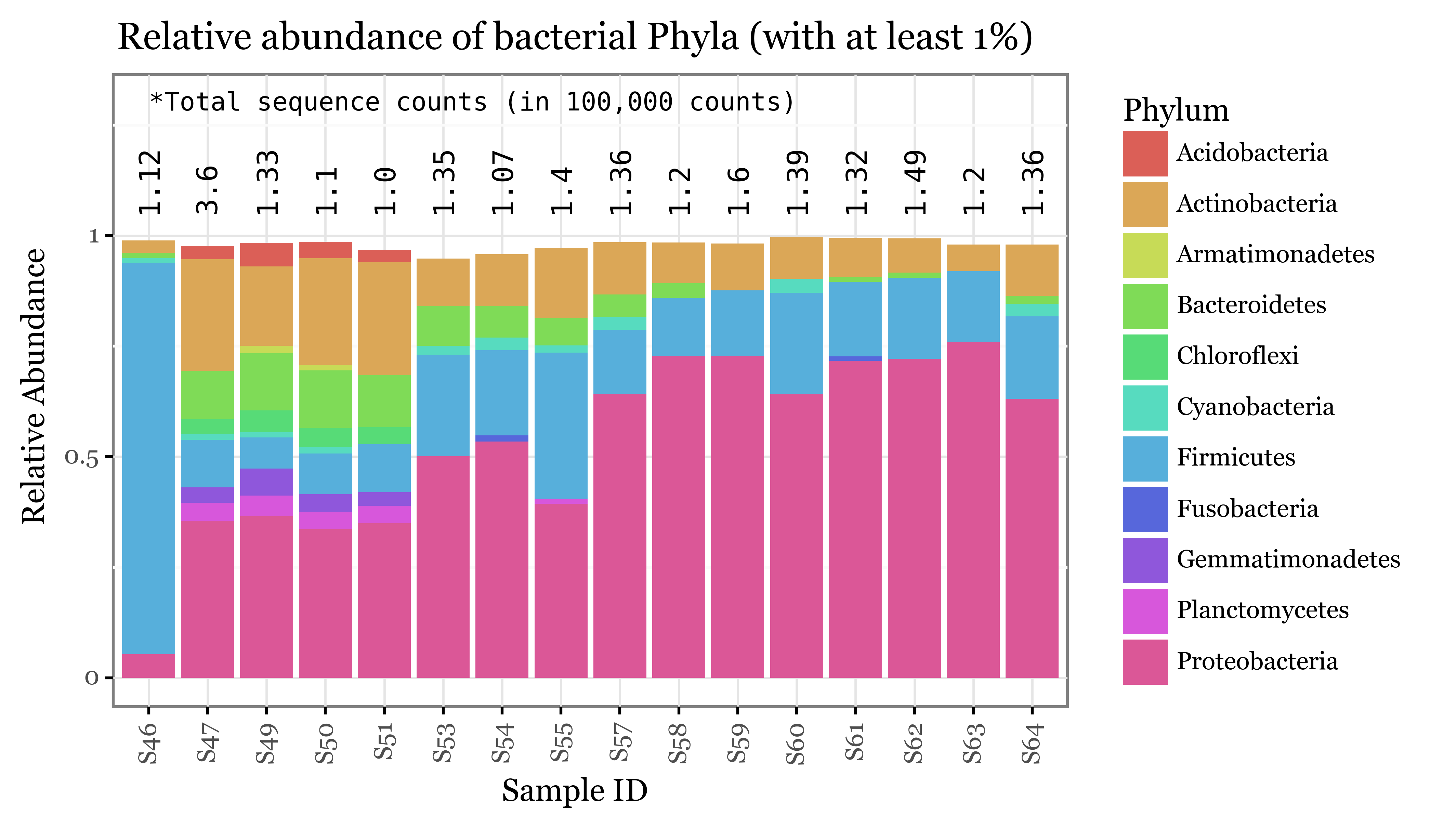
abundance_per_week = subdaily_samples.groupby(['Kingdom', 'sample_id']).abundance.sum()abundance_per_week.loc['Bacteria', 'S46']112211.0taxons['Kingdom', 'Phylum', 'Class', 'Order', 'Family', 'Genus', 'Species']kingdom = 'Bacteria'
(subdaily_samples
.loc[lambda dd: dd.Kingdom==kingdom]
.groupby(['sample_id', 'Phylum'], as_index=False)
.abundance.sum()
.assign(frequency=lambda dd: [c / abundance_per_week.loc[kingdom, s] for c, s in zip(dd['abundance'], dd['sample_id'])])
.loc[lambda dd: dd['frequency'] > .01]
.pipe(lambda dd: p9.ggplot(dd)
+ p9.aes('sample_id', 'frequency', fill='Phylum')
+ p9.geom_col()
+ p9.geom_text(data=abundance_per_week.loc[kingdom].reset_index().loc[lambda dd: dd.abundance>0].assign(countstr=lambda dd: (dd['abundance'] / 1e5).round(2)),
color='black', angle=90, size=10, family='monospace', y=1.05, mapping=p9.aes(x='sample_id', label='countstr'), inherit_aes=False, va='bottom')
+ p9.theme_bw()
+ p9.annotate('text', x=1, y=1.3, size=9, label='*Total sequence counts (in 100,000 counts)', family='monospace', ha='left')
+ p9.theme(axis_text_x=p9.element_text(rotation=90, hjust=.5))
+ p9.labs(x='Sample ID', y='Relative Abundance', color='Phyla', title=f'Relative abundance of bacterial Phyla (with at least 1%)')
+ p9.theme(dpi=300, figure_size=(6, 4))
))
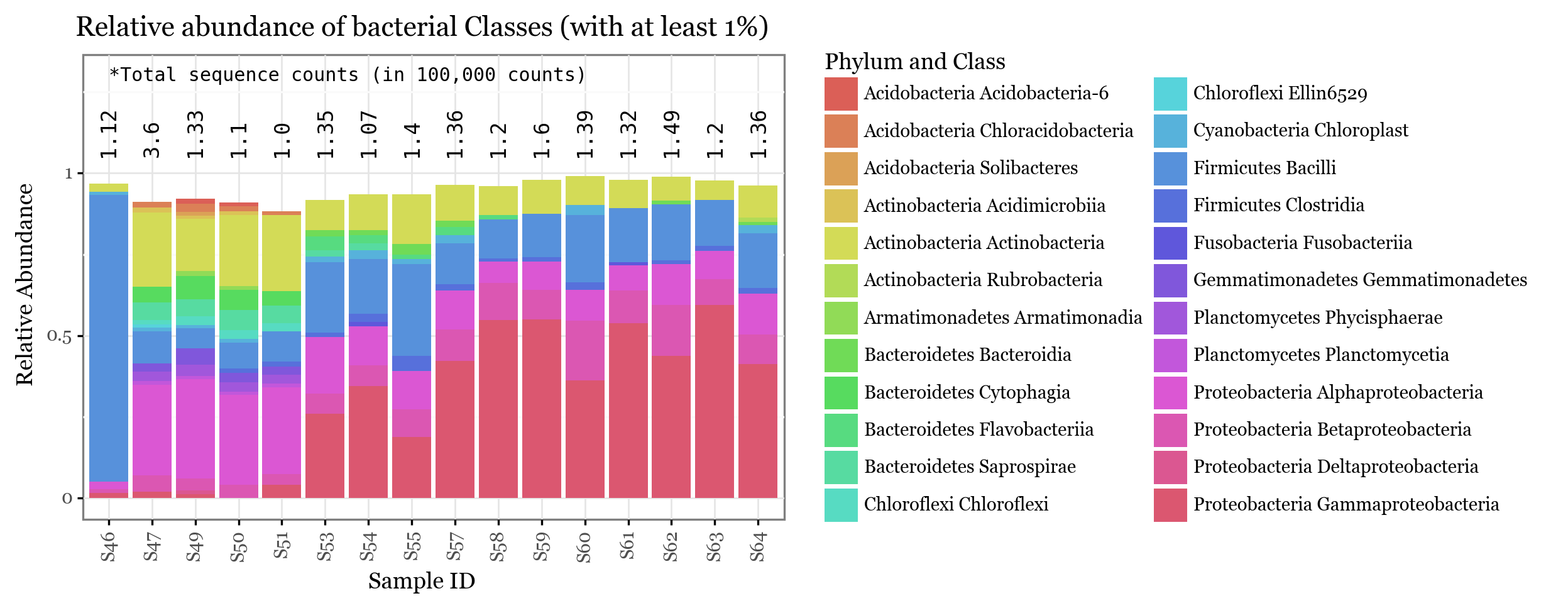
kingdom = 'Bacteria'
(subdaily_samples
 .loc[lambda dd: dd.Kingdom==kingdom]
 .groupby(['sample_id', 'Phylum', 'Class'], as_index=False)
 .abundance.sum()
 .assign(frequency=lambda dd: [c / abundance_per_week.loc[kingdom, s] for c, s in zip(dd['abundance'], dd['sample_id'])])
 .assign(phylclass=lambda dd:  dd.Phylum + ' ' + dd.Class)
 .loc[lambda dd: dd['frequency'] > .01]
 .pipe(lambda dd: p9.ggplot(dd)
      + p9.aes('sample_id', 'frequency', fill='phylclass')
      + p9.geom_col()
      + p9.geom_text(data=abundance_per_week.loc[kingdom].reset_index().loc[lambda dd: dd.abundance>0].assign(countstr=lambda dd: (dd['abundance'] / 1e5).round(2)),
                     color='black', angle=90, size=10, family='monospace', y=1.05, mapping=p9.aes(x='sample_id', label='countstr'), inherit_aes=False, va='bottom')
      + p9.theme_bw()
      + p9.annotate('text', x=1, y=1.3, size=9, label='*Total sequence counts (in 100,000 counts)', family='monospace', ha='left')
      + p9.theme(axis_text_x=p9.element_text(rotation=90, hjust=.5))
      + p9.labs(x='Sample ID', y='Relative Abundance', color='phylclass', title=f'Relative abundance of bacterial Classes (with at least 1%)', fill='Phylum and Class')
      + p9.theme(dpi=120, figure_size=(6, 4))
))
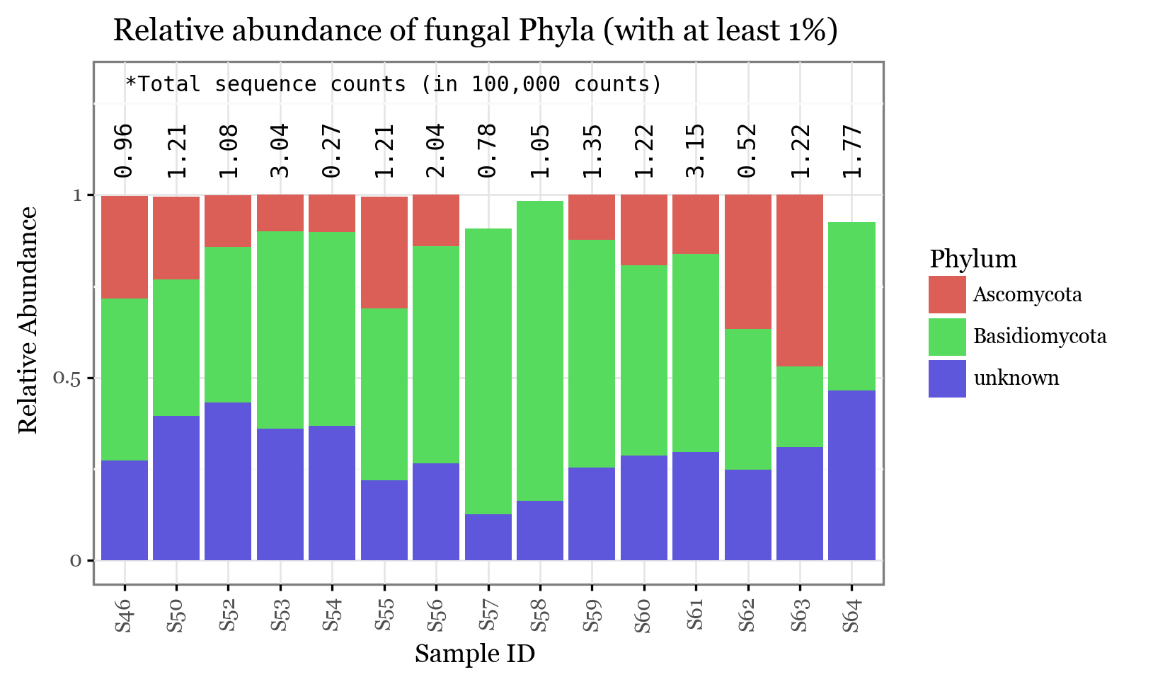
kingdom = 'Fungi'
(subdaily_samples
 .loc[lambda dd: dd.Kingdom==kingdom]
 .groupby(['sample_id', 'Phylum'], as_index=False)
 .abundance.sum()
 .assign(frequency=lambda dd: [c / abundance_per_week.loc[kingdom, s] for c, s in zip(dd['abundance'], dd['sample_id'])])
 .loc[lambda dd: dd['frequency'] > .1]
 .pipe(lambda dd: p9.ggplot(dd)
      + p9.aes('sample_id', 'frequency', fill='Phylum')
      + p9.geom_col()
      + p9.geom_text(data=abundance_per_week.loc[kingdom].reset_index().loc[lambda dd: dd.abundance > 0].assign(countstr=lambda dd: (dd['abundance'] / 1e5).round(2)),
                     color='black', angle=90, size=10, family='monospace', y=1.05, mapping=p9.aes(x='sample_id', label='countstr'), inherit_aes=False, va='bottom')
      + p9.theme_bw()
      + p9.annotate('text', x=1, y=1.3, size=9, label='*Total sequence counts (in 100,000 counts)', family='monospace', ha='left')
      + p9.theme(axis_text_x=p9.element_text(rotation=90, hjust=.5))
      + p9.labs(x='Sample ID', y='Relative Abundance', color='Phyla', title=f'Relative abundance of fungal Phyla (with at least 1%)')
      + p9.theme(dpi=120, figure_size=(6, 4))
))
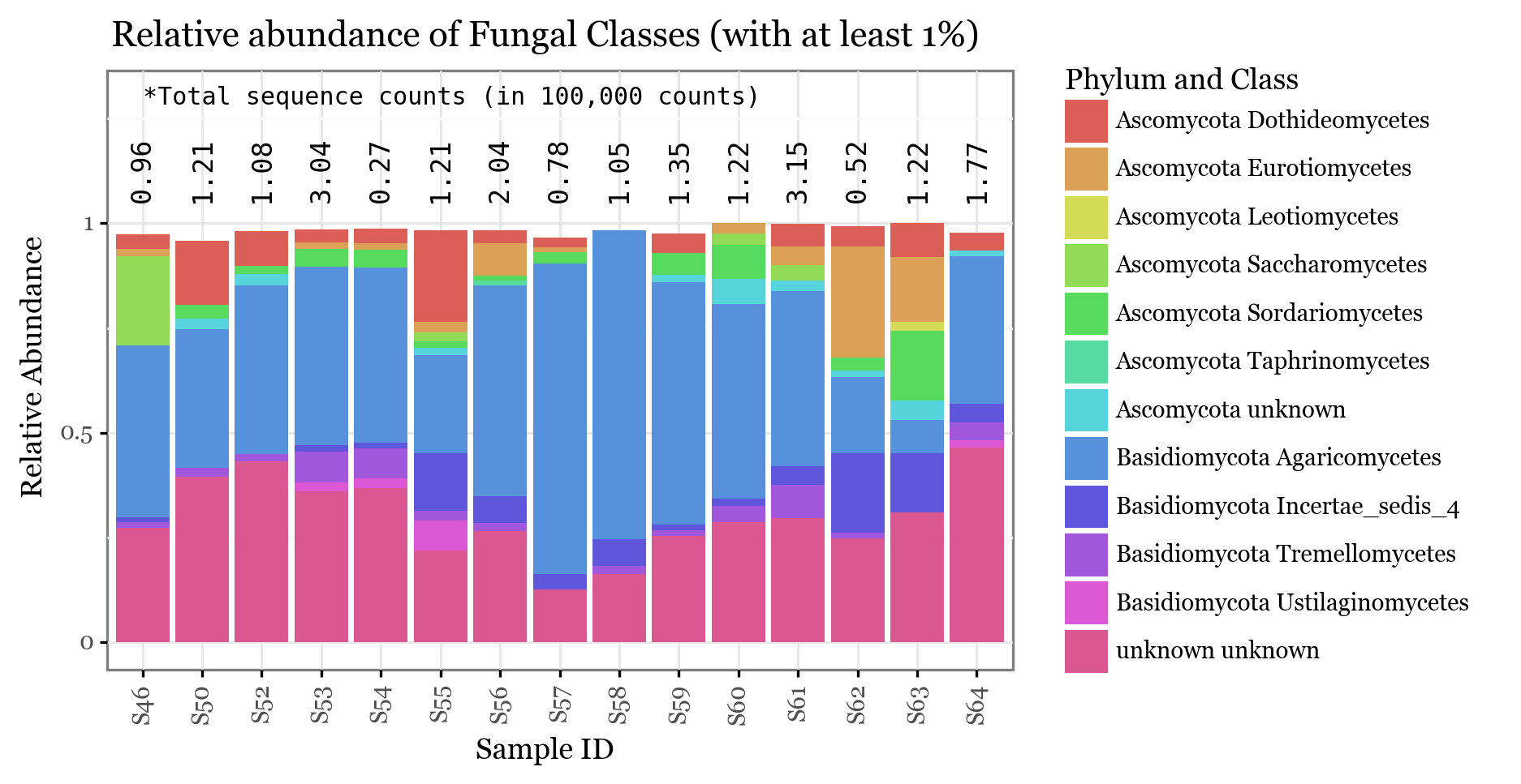
kingdom = 'Fungi'
(subdaily_samples
 .loc[lambda dd: dd.Kingdom==kingdom]
 .groupby(['sample_id', 'Phylum', 'Class'], as_index=False)
 .abundance.sum()
 .assign(frequency=lambda dd: [c / abundance_per_week.loc[kingdom, s] for c, s in zip(dd['abundance'], dd['sample_id'])])
 .assign(phylclass=lambda dd:  dd.Phylum + ' ' + dd.Class)
 .loc[lambda dd: dd['frequency'] > .01]
 .pipe(lambda dd: p9.ggplot(dd)
      + p9.aes('sample_id', 'frequency', fill='phylclass')
      + p9.geom_col()
      + p9.geom_text(data=abundance_per_week.loc[kingdom].reset_index().loc[lambda dd: dd.abundance>0].assign(countstr=lambda dd: (dd['abundance'] / 1e5).round(2)),
                     color='black', angle=90, size=10, family='monospace', y=1.05, mapping=p9.aes(x='sample_id', label='countstr'), inherit_aes=False, va='bottom')
      + p9.theme_bw()
      + p9.annotate('text', x=1, y=1.3, size=9, label='*Total sequence counts (in 100,000 counts)', family='monospace', ha='left')
      + p9.theme(axis_text_x=p9.element_text(rotation=90))
      + p9.labs(x='Sample ID', y='Relative Abundance', color='phylclass', title=f'Relative abundance of Fungal Classes (with at least 1%)', fill='Phylum and Class')
      + p9.theme(dpi=120, figure_size=(6, 4))
))
Diversity
def bray_curtis_similarity(a, b):
    C = np.min([a, b], axis=0).sum()
    S = np.sum([a, b])
    return C * 2 / S
sample_type_dict = (subdaily_samples
.loc[lambda dd: dd.Kingdom.isin(['Bacteria', 'Fungi'])]
.loc[lambda dd: dd.abundance > 0]
.groupby('sample_id')
.Kingdom
.unique()
.str.join('-')
.reset_index()
.groupby('Kingdom')
.agg(lambda x: list(x))
.to_dict()
['sample_id']
)
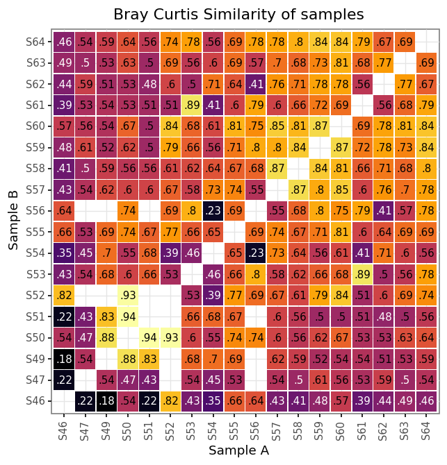
{'Bacteria': ['S47', 'S49', 'S51'], 'Bacteria-Fungi': ['S46', 'S50', 'S53', 'S54', 'S55', 'S57', 'S58', 'S59', 'S60', 'S61', 'S62', 'S63', 'S64'], 'Fungi': ['S52', 'S56']}Since not all samples contain information for both Bacteria and Fungi, we cannot consider all Phyla as possible when calculating the Bray Curtis similarity or it would lead us to artificially low values for those pairs of samples for which the set of evaluated Phyla was not the same. In order to correct for this, what we will do is 3 different comparisons and aggregate as follows:
- Samples with successfull ITS and 16S sequencing will be compared using the whole set of Bacterial and Fungal Phyla only among themselves.
- Samples only successful on 16S sequencing will be compared to other 16S-only samples and 16S + ITS samples on the Bacterial Phyla set.
- Samples only successful on ITS sequencing will be compared to other ITS-only samples and 16S + ITS samples on the Fungal Phyla set.
- There will be no comparison among ITS-only and 16S only samples, since there is no common set to make the comparison.
Raw
bc_both = (subdaily_samples
                 .loc[lambda dd: dd.Kingdom.isin(['Bacteria', 'Fungi'])]
                 .loc[lambda dd: dd.sample_id.isin(sample_type_dict['Bacteria-Fungi'])]
                 .groupby(['sample_id', 'Phylum'], as_index=False)
                 .abundance.sum()
                 .pivot('Phylum', 'sample_id', 'abundance')
                 .corr(method=bray_curtis_similarity)
                 .reset_index()
                 .rename(columns={'sample_id': 'sample_id_a'})
                 .melt('sample_id_a', var_name='sample_id_b', value_name='bray_curtis_similarity')
                 .loc[lambda dd: dd.sample_id_a != dd.sample_id_b])
bc_fungi = (subdaily_samples
.loc[lambda dd: dd.Kingdom.isin(['Bacteria', 'Fungi'])]
.loc[lambda dd: dd.sample_id != 'S48']
.loc[lambda dd: ~dd.sample_id.isin(sample_type_dict['Bacteria'])]
.loc[lambda dd: dd.Kingdom=='Fungi']
.groupby(['sample_id', 'Phylum'], as_index=False)
.abundance.sum()
.pivot('Phylum', 'sample_id', 'abundance')
.corr(method=bray_curtis_similarity)
.reset_index()
.rename(columns={'sample_id': 'sample_id_a'})
.melt('sample_id_a', var_name='sample_id_b', value_name='bray_curtis_similarity')
.loc[lambda dd: dd.sample_id_a != dd.sample_id_b]
.loc[lambda dd: (dd.sample_id_a.isin(sample_type_dict['Fungi'])) | (dd.sample_id_b.isin(sample_type_dict['Fungi']))]
)bc_bacteria = (subdaily_samples
.loc[lambda dd: dd.Kingdom.isin(['Bacteria', 'Fungi'])]
.loc[lambda dd: dd.sample_id != 'S48']
.loc[lambda dd: ~dd.sample_id.isin(sample_type_dict['Fungi'])]
.loc[lambda dd: dd.Kingdom=='Bacteria']
.groupby(['sample_id', 'Phylum'], as_index=False)
.abundance.sum()
.pivot('Phylum', 'sample_id', 'abundance')
.corr(method=bray_curtis_similarity)
.reset_index()
.rename(columns={'sample_id': 'sample_id_a'})
.melt('sample_id_a', var_name='sample_id_b', value_name='bray_curtis_similarity')
.loc[lambda dd: dd.sample_id_a != dd.sample_id_b]
.loc[lambda dd: (dd.sample_id_a.isin(sample_type_dict['Bacteria'])) | (dd.sample_id_b.isin(sample_type_dict['Bacteria']))]
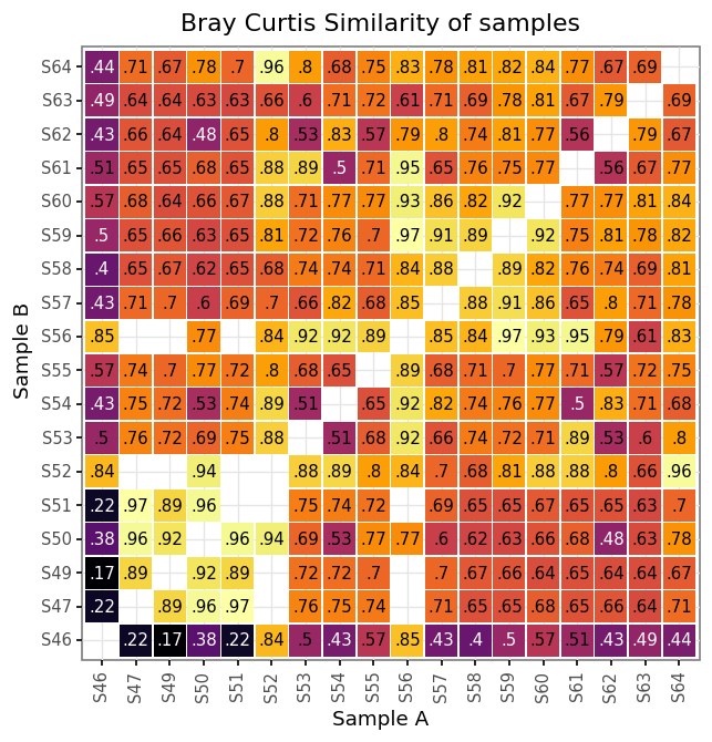
)samples_bc = pd.concat([bc_bacteria, bc_fungi, bc_both])(samples_bc
.assign(bc_str=lambda dd: dd.bray_curtis_similarity.round(2).astype(str).str[1:])
.pipe(lambda dd: p9.ggplot(dd)
+ p9.aes(x='sample_id_a', y='sample_id_b', fill='bray_curtis_similarity')
+ p9.geom_tile(p9.aes(width=.95, height=.95))
+ p9.geom_text(p9.aes(label='bc_str', color='bray_curtis_similarity > .5'), size=9)
+ p9.scale_color_manual(['white', 'black'])
+ p9.theme_bw()
+ p9.scale_fill_continuous('inferno')
+ p9.theme(dpi=120, figure_size=(6, 6), axis_text_x=p9.element_text(rotation=90))
+ p9.labs(x='Sample A', y='Sample B', title='Bray Curtis Similarity of samples')
+ p9.guides(fill=False, color=False))
)
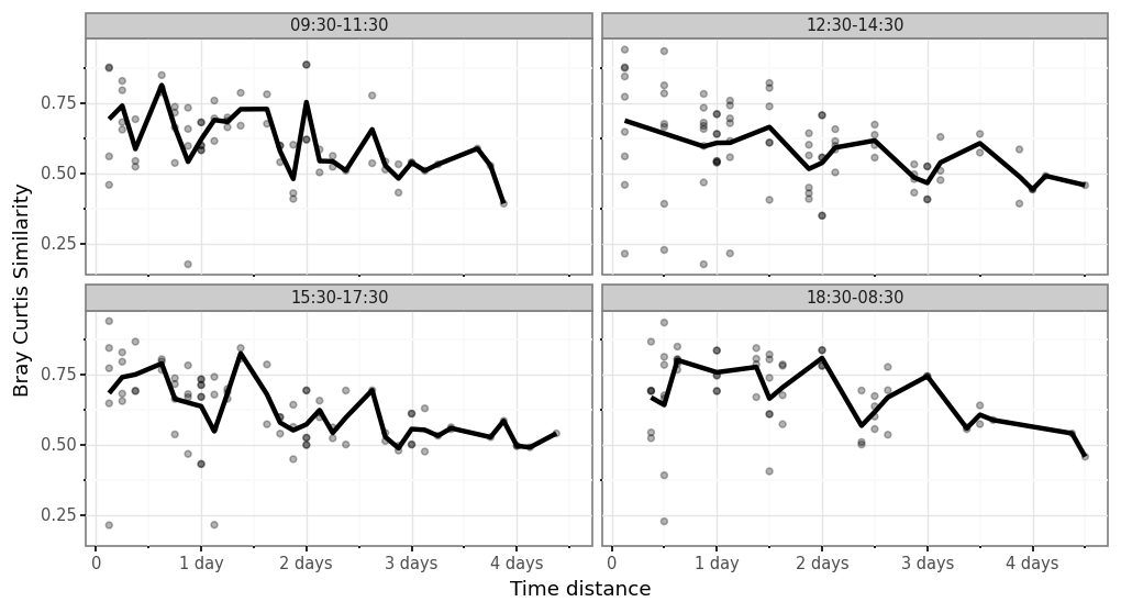
(samples_bc
 .merge(samples_info.set_index('sample_id'), left_on='sample_id_a', right_index=True)
 .merge(samples_info.set_index('sample_id'), left_on='sample_id_b', right_index=True, suffixes=('_a', '_b'))
 .assign(time_delta=lambda dd: abs(dd.centroid_a - dd.centroid_b))
 .pipe(lambda dd: p9.ggplot(dd)
       + p9.aes('time_delta', 'bray_curtis_similarity')
       + p9.geom_point(alpha=.3)
       + p9.theme_bw()
       + p9.theme(dpi=120, figure_size=(10, 5))
       + p9.facet_wrap('time_slot_a', ncol=2)
       + p9.stat_summary(fun_y=np.mean, geom='line', size=1.5)
       + p9.labs(x='Time distance', y='Bray Curtis Similarity'))
)
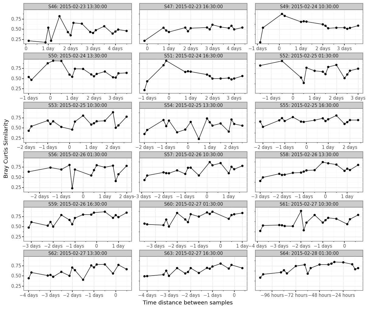
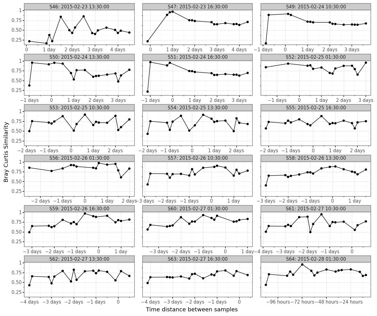
(samples_bc
 .merge(samples_info.set_index('sample_id'), left_on='sample_id_a', right_index=True)
 .merge(samples_info.set_index('sample_id'), left_on='sample_id_b', right_index=True, suffixes=('_a', '_b'))
 .assign(time_delta=lambda dd: dd.centroid_b - dd.centroid_a)
 .assign(sample_str=lambda dd: dd.sample_id_a + ': ' + dd.centroid_a.astype(str))
 .pipe(lambda dd: p9.ggplot(dd)
       + p9.aes('time_delta', 'bray_curtis_similarity')
       + p9.geom_point()
       + p9.geom_line()
       + p9.theme_bw()
       + p9.theme(dpi=120, figure_size=(12, 10), subplots_adjust={'hspace': 0.45, 'wspace': .075})
       + p9.facet_wrap('sample_str', ncol=3, scales='free_x')
       + p9.labs(x='Time distance between samples', y='Bray Curtis Similarity')
      )
)
Normalized
bc_both_norm = (subdaily_samples
                 .loc[lambda dd: dd.Kingdom.isin(['Bacteria', 'Fungi'])]
                 .loc[lambda dd: dd.sample_id.isin(sample_type_dict['Bacteria-Fungi'])]
                 .groupby(['sample_id', 'Phylum'], as_index=False)
                 .abundance.sum()
                 .pivot('Phylum', 'sample_id', 'abundance')
                 .apply(lambda x: x / x.max())
                 .corr(method=bray_curtis_similarity)
                 .reset_index()
                 .rename(columns={'sample_id': 'sample_id_a'})
                 .melt('sample_id_a', var_name='sample_id_b', value_name='bray_curtis_similarity')
                 .loc[lambda dd: dd.sample_id_a != dd.sample_id_b])
bc_fungi_norm = (subdaily_samples
.loc[lambda dd: dd.Kingdom.isin(['Bacteria', 'Fungi'])]
.loc[lambda dd: dd.sample_id != 'S48']
.loc[lambda dd: ~dd.sample_id.isin(sample_type_dict['Bacteria'])]
.loc[lambda dd: dd.Kingdom=='Fungi']
.groupby(['sample_id', 'Phylum'], as_index=False)
.abundance.sum()
.pivot('Phylum', 'sample_id', 'abundance')
.apply(lambda x: x / x.max())
.corr(method=bray_curtis_similarity)
.reset_index()
.rename(columns={'sample_id': 'sample_id_a'})
.melt('sample_id_a', var_name='sample_id_b', value_name='bray_curtis_similarity')
.loc[lambda dd: dd.sample_id_a != dd.sample_id_b]
.loc[lambda dd: (dd.sample_id_a.isin(sample_type_dict['Fungi'])) | (dd.sample_id_b.isin(sample_type_dict['Fungi']))]
)bc_bacteria_norm = (subdaily_samples
.loc[lambda dd: dd.Kingdom.isin(['Bacteria', 'Fungi'])]
.loc[lambda dd: dd.sample_id != 'S48']
.loc[lambda dd: ~dd.sample_id.isin(sample_type_dict['Fungi'])]
.loc[lambda dd: dd.Kingdom=='Bacteria']
.groupby(['sample_id', 'Phylum'], as_index=False)
.abundance.sum()
.pivot('Phylum', 'sample_id', 'abundance')
.apply(lambda x: x / x.max())
.corr(method=bray_curtis_similarity)
.reset_index()
.rename(columns={'sample_id': 'sample_id_a'})
.melt('sample_id_a',
var_name='sample_id_b',
value_name='bray_curtis_similarity')
.loc[lambda dd: dd.sample_id_a != dd.sample_id_b]
.loc[lambda dd: (dd.sample_id_a.isin(sample_type_dict['Bacteria']))
| (dd.sample_id_b.isin(sample_type_dict['Bacteria']))]
)samples_bc_norm = pd.concat([bc_bacteria_norm, bc_fungi_norm, bc_both_norm])(samples_bc_norm
.assign(bc_str=lambda dd: dd.bray_curtis_similarity.round(2).astype(str).str[1:])
.pipe(lambda dd: p9.ggplot(dd)
+ p9.aes(x='sample_id_a', y='sample_id_b', fill='bray_curtis_similarity')
+ p9.geom_tile(p9.aes(width=.95, height=.95))
+ p9.geom_text(p9.aes(label='bc_str', color='bray_curtis_similarity > .5'), size=9)
+ p9.scale_color_manual(['white', 'black'])
+ p9.theme_bw()
+ p9.scale_fill_continuous('inferno')
+ p9.theme(dpi=120, figure_size=(6, 6), axis_text_x=p9.element_text(rotation=90))
+ p9.labs(x='Sample A', y='Sample B', title='Bray Curtis Similarity of samples')
+ p9.guides(fill=False, color=False))
)
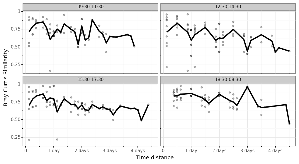
(samples_bc_norm
 .merge(samples_info.set_index('sample_id'), left_on='sample_id_a', right_index=True)
 .merge(samples_info.set_index('sample_id'), left_on='sample_id_b', right_index=True, suffixes=('_a', '_b'))
 .assign(time_delta=lambda dd: abs(dd.centroid_b - dd.centroid_a))
 .pipe(lambda dd: p9.ggplot(dd)
       + p9.aes('time_delta', 'bray_curtis_similarity')
       + p9.geom_point(alpha=.3)
       + p9.theme_bw()
       + p9.theme(dpi=120, figure_size=(10, 5))
       + p9.facet_wrap('time_slot_a', ncol=2)
       + p9.stat_summary(fun_y=np.mean, geom='line', size=1.5)
       + p9.labs(x='Time distance', y='Bray Curtis Similarity'))
)
(samples_bc_norm
 .merge(samples_info.set_index('sample_id'), left_on='sample_id_a', right_index=True)
 .merge(samples_info.set_index('sample_id'), left_on='sample_id_b', right_index=True, suffixes=('_a', '_b'))
 .assign(time_delta=lambda dd: dd.centroid_b - dd.centroid_a)
 .assign(sample_str=lambda dd: dd.sample_id_a + ': ' + dd.centroid_a.astype(str))
 .pipe(lambda dd: p9.ggplot(dd)
       + p9.aes('time_delta', 'bray_curtis_similarity')
       + p9.geom_point()
       + p9.geom_line()
       + p9.theme_bw()
       + p9.theme(dpi=120, figure_size=(12, 10), subplots_adjust={'hspace': 0.45, 'wspace': .075})
       + p9.facet_wrap('sample_str', ncol=3, scales='free_x')
       + p9.labs(x='Time distance between samples', y='Bray Curtis Similarity')
      )
)
Metals
pd.options.display.max_columns = 999
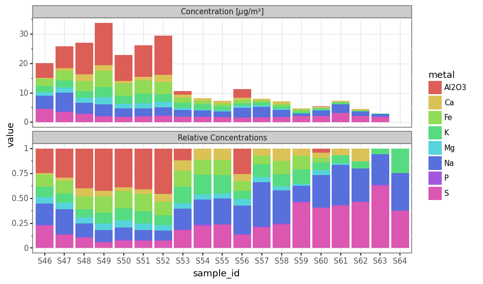
micro_metals = subdaily_metals.index.values[3:11]
micro_metalsarray(['Al2O3', 'Ca', 'Fe', 'K', 'Mg', 'Na', 'P', 'S'], dtype=object)subdaily_metals = (subdaily_metals
.T
.iloc[1:]
.loc[samples_info.sample_id]
.drop(columns=['Initial', 'Final', 'm3'])
.replace({'<dl': 0})
.reset_index()
.rename(columns={'index': 'sample_id'})
.melt('sample_id', var_name='metal', value_name='concentration')
.assign(concentration=lambda dd: np.where(dd.metal.isin(micro_metals), dd.concentration, dd.concentration / 1000))
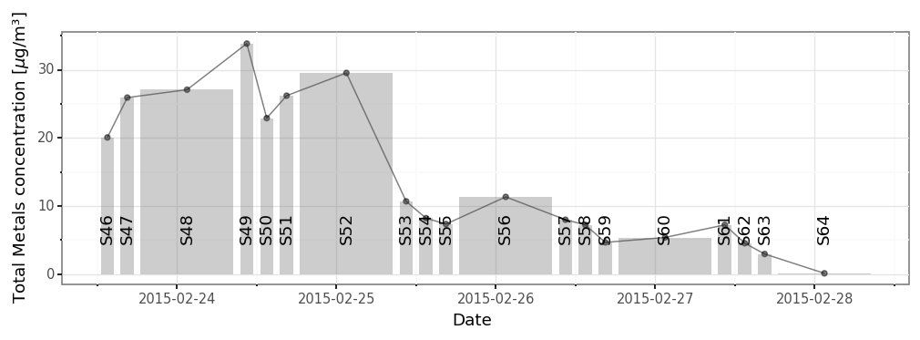
)(subdaily_metals
.loc[lambda dd: dd.metal.isin(micro_metals)]
#.loc[lambda dd: dd.metal != 'Al2O3']
.groupby('sample_id')
.concentration
.sum()
.rename('total_concentration')
.reset_index()
.merge(samples_info)
.pipe(lambda dd: p9.ggplot(dd)
+ p9.geom_line(p9.aes(x='initial + (final - initial) / 2', y='total_concentration'), alpha=.5)
+ p9.geom_point(p9.aes(x='initial + (final - initial) / 2', y='total_concentration'), alpha=.5)
+ p9.geom_rect(mapping=p9.aes(xmin='initial', xmax='final', ymax='total_concentration'), ymin=0, alpha=.3)
+ p9.geom_text(p9.aes(label='sample_id', x='initial + (final - initial) / 2'), angle=90, y=dd.total_concentration.max() / 5)
+ p9.theme_bw()
+ p9.theme(dpi=120, figure_size=(10, 3))
+ p9.labs(x='Date', y=r'Total Metals concentration [$\mu$g/m³]'))
)
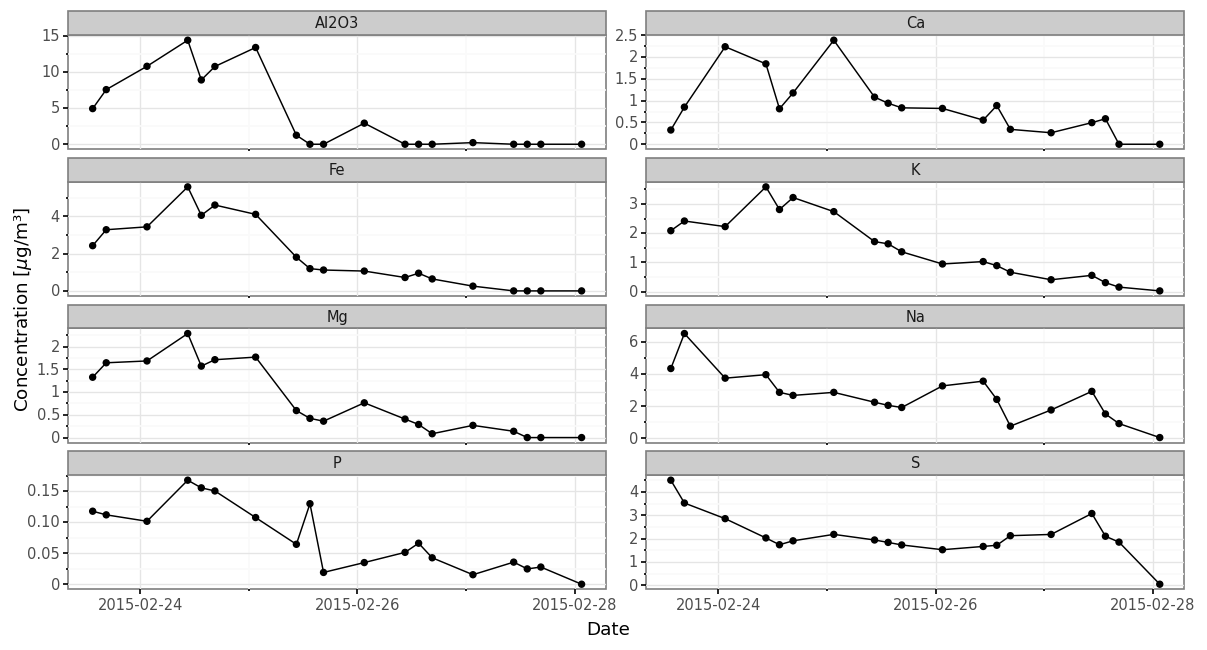
from mizani.breaks import date_breaks(subdaily_metals
.loc[lambda dd: dd.metal.isin(micro_metals)]
.merge(samples_info)
.pipe(lambda dd: p9.ggplot(dd)
+ p9.aes('initial + (final - initial) / 2', 'concentration')
+ p9.geom_line(group='metal')
+ p9.geom_point()
+ p9.theme_bw()
+ p9.scale_x_datetime(breaks=date_breaks('2 days'))
+ p9.theme(dpi=120, figure_size=(12, 6), subplots_adjust={'wspace':0.075})
+ p9.facet_wrap('metal', scales='free_y', ncol=2)
+ p9.labs(x='Date', y=r'Concentration [$\mu$g/m³]'))
)
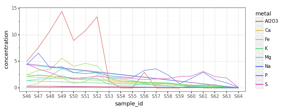
(subdaily_metals
  .loc[lambda dd: dd.metal.isin(micro_metals)]
  .pipe(lambda dd: p9.ggplot(dd)
        + p9.aes('sample_id', 'concentration', color='metal')
        + p9.geom_line(group='metal')
        + p9.theme_bw()
        + p9.theme(dpi=120, figure_size=(8, 3)))
)
total_metals_per_sample = subdaily_metals.loc[lambda dd: dd.metal.isin(micro_metals)].groupby('sample_id').concentration.sum()
(subdaily_metals
  .loc[lambda dd: dd.metal.isin(micro_metals)]
  .assign(value=lambda dd: [c / total_metals_per_sample.loc[s] for c, s in zip(dd.concentration, dd.sample_id)])
  .assign(kind='Relative Concentrations')
  [['sample_id', 'value', 'metal', 'kind']]
  .pipe(lambda dd: pd.concat([dd, subdaily_metals.loc[lambda dd: dd.metal.isin(micro_metals)].assign(kind=r'Concentration [$\mu$g/m³]', value=lambda dd: dd.concentration)]))
  .pipe(lambda dd: p9.ggplot(dd)
        + p9.aes('sample_id', 'value', fill='metal')
        + p9.geom_col(group='metal')
        + p9.theme_bw()
        + p9.facet_wrap('kind', ncol=1, scales='free_y')
        + p9.theme(dpi=120, figure_size=(8, 5)))
)
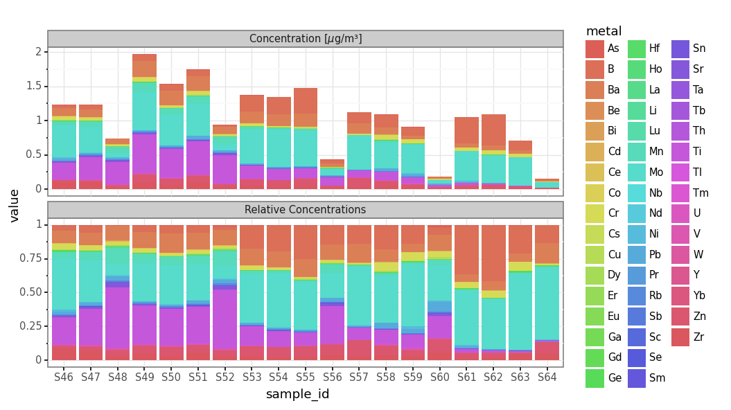
total_metals_per_sample = subdaily_metals.loc[lambda dd: ~dd.metal.isin(micro_metals)].groupby('sample_id').concentration.sum()
(subdaily_metals
  .loc[lambda dd: ~dd.metal.isin(micro_metals)]
  .assign(value=lambda dd: [c / total_metals_per_sample.loc[s] for c, s in zip(dd.concentration, dd.sample_id)])
  .assign(kind='Relative Concentrations')
  [['sample_id', 'value', 'metal', 'kind']]
  .pipe(lambda dd: pd.concat([dd, subdaily_metals.loc[lambda dd: ~dd.metal.isin(micro_metals)].assign(kind=r'Concentration [$\mu$g/m³]', value=lambda dd: dd.concentration)]))
  .pipe(lambda dd: p9.ggplot(dd)
        + p9.aes('sample_id', 'value', fill='metal')
        + p9.geom_col(group='metal')
        + p9.theme_bw()
        + p9.facet_wrap('kind', ncol=1, scales='free_y')
        + p9.theme(dpi=120, figure_size=(8, 5)))
)
References
- [1] Gusareva, E. S., Acerbi, E., Lau, K. J., Luhung, I., Premkrishnan, B. N., Kolundžija, S., … & Gaultier, N. E. (2019). Microbial communities in the tropical air ecosystem follow a precise diel cycle. Proceedings of the National Academy of Sciences, 116(46), 23299-23308. https://www.pnas.org/content/116/46/23299
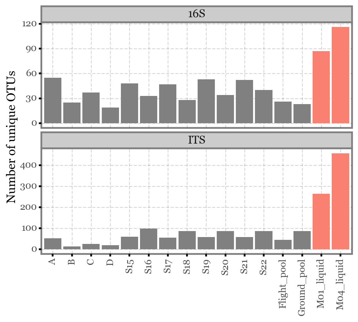
from collections import defaultdictcols = ['Global', 'A', 'B', 'C', 'D', 'S15', 'S16', 'S17', 'S18', 'S19',
'S20', 'S21', 'S22', 'Flight_pool', 'Ground_pool', 'M01_liquid', 'M04_liquid']
data = defaultdict(list)
for i, col in enumerate(cols):
data['col'].append(col)
df_its = pd.read_excel('/Users/alfontal/Downloads/Resum_ITS.xlsx', sheet_name=i)
df_16s = pd.read_excel('/Users/alfontal/Downloads/Resum_16S.xlsx', sheet_name=i)
data['alpha_ITS'].append(df_its.shape[0] - 1)
data['alpha_16S'].append(df_16s.shape[0] - 1)i16(pd.DataFrame(data).iloc[1:]
.reset_index()
.melt(['col', 'index'])
.assign(extra=lambda dd: np.where(dd.col.str.contains('liquid'), 'liquid', 'filter'))
.assign(col=lambda dd: pd.Categorical(dd.col, categories=dd.col[:16], ordered=True))
.assign(variable=lambda dd: dd.variable.str.replace('alpha_', ''))
.pipe(lambda dd: p9.ggplot(dd)
+ p9.aes('col', 'value', fill='variable')
+ p9.geom_col(p9.aes(fill='extra'))
+ p9.facet_wrap('variable', ncol=1, scales='free_y')
+ p9.labs(x='', y='Number of unique OTUs')
+ p9.scale_fill_manual(['gray', 'salmon'])
+ p9.guides(fill=False)
+ p9.theme(axis_text_x=p9.element_text(rotation=90))
)
)